Static Map Tab

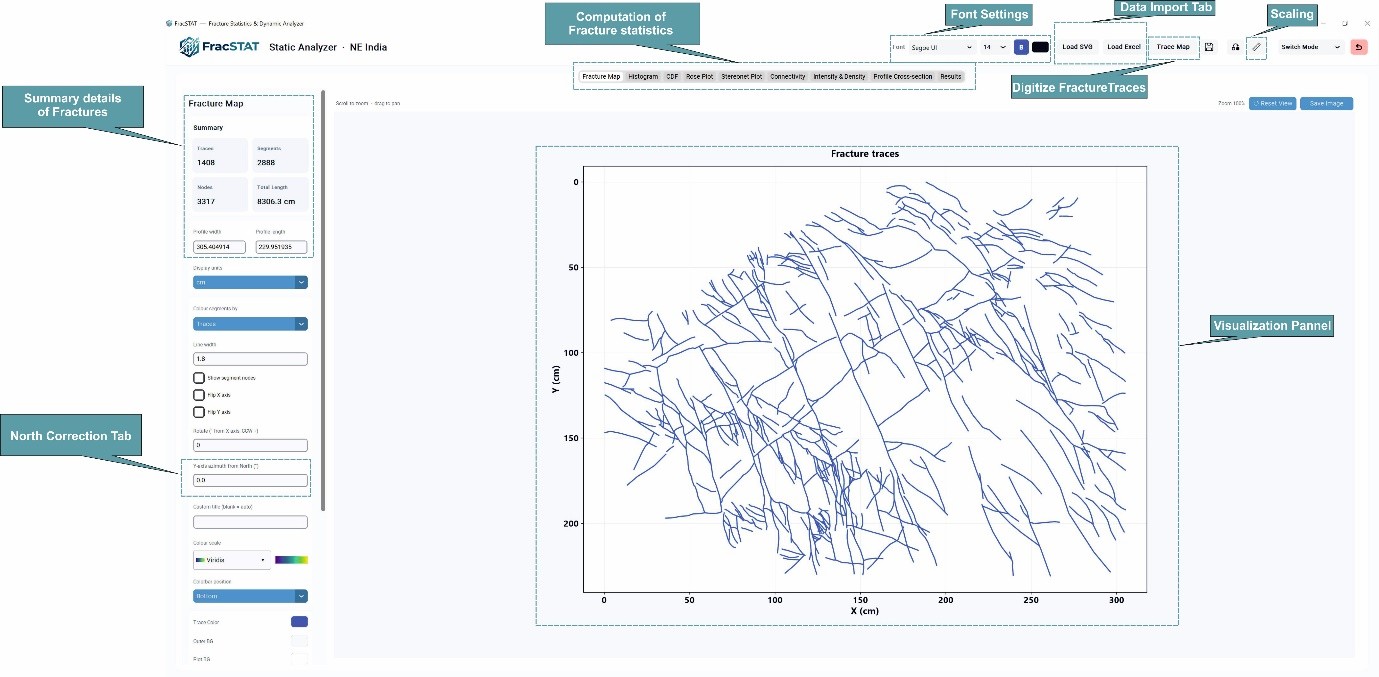
Located at static_analyzer/tabs/static_map_tab.py, the Fracture Map tab (referred to as the "Static Map Tab" in the technical reference) is the first thing you see after importing fracture data into FracSTAT's Static Module. It draws a two‑dimensional, publication‑style plan‑view map of your fracture network, and it is the visual foundation that every other statistical tab (Histogram, CDF, Rose, Stereonet, Connectivity, Intensity, Profile, Results) builds on. This guide walks a complete beginner through everything: how to get data onto the map, what every control in the sidebar does, the maths running underneath, and how to read the finished map geologically.

1. Getting Fracture Data Onto the Map

Before the Fracture Map tab has anything to show, a fracture dataset has to be prepared inside the Static Module. FracSTAT accepts fracture data from three different sources, so you can bring in whatever you already have:

• Outcrop images with a referenced scale, digitized inside FracSTAT itself.
• SVG files — fracture traces already digitized in a vector‑graphics program such as Adobe Illustrator, CorelDraw, or Inkscape.
• Tabulated data (Excel/CSV) — spreadsheets containing Fracture ID, strike, dip, length, aperture and similar attributes.

Figure 2.1 — GUI of the Static Analyzer module showing the data‑import options, from which users can import, prepare and statistically analyse fracture traces.

1.1 Load SVG

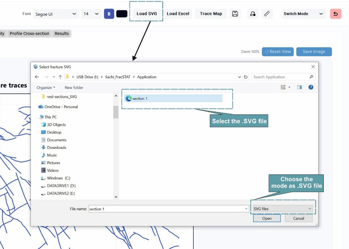
If your fracture traces are already digitized and saved as an .svg file, click the Load SVG tab and select the file. FracSTAT reads the file with core.svg_loader.read_svg_segments(), converting every curve into short straight segments (a "curve step" of 12 pixels is used internally) so the geometry can be processed the same way as hand‑digitized traces. This lets you bring existing fracture maps straight into the analysis workflow without any extra pre‑processing.

Figure 2.2 — Data import using the "Load SVG" tab. Once clicked, users select an SVG file and it is uploaded to the GUI.

1.2 Load Excel

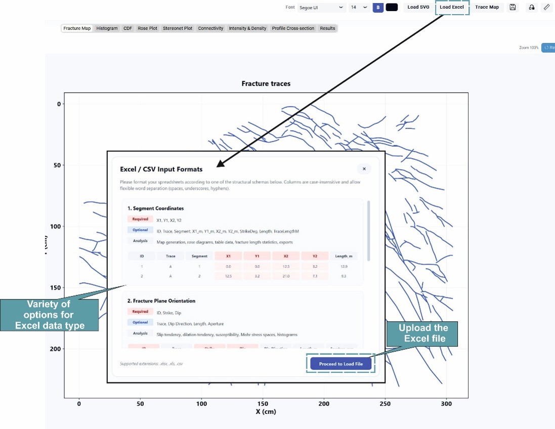
If your fracture information already exists as a spreadsheet or CSV, use the Load Excel option instead of digitizing anything. The file is parsed by core.excel_loader.read_excel_segments(), which auto‑detects which of five supported layouts your file matches — purely from its column headers. Column names are matched case‑insensitively, and spaces, hyphens and underscores are ignored, so "Dip Direction", "dip_direction" and "DipDirection" are all read the same way. Any extra columns your file happens to contain are simply ignored. Any unrecognised rows are skipped rather than crashing the whole import.

How to read the tables below:

Format 1 — Segment Coordinates

Real‑world endpoint coordinates for each segment. This is also the format FracSTAT's own exported results use, so a file you exported earlier can be re‑imported directly. Segments loaded this way are flagged internally to keep their real‑world 1:1 scale, exactly like spatial Excel/CSV data described in Section 8.1 — no rescaling to a profile box is applied.

ID	Trace	Segment	X1	Y1	X2	Y2	Length_m
1	A	1	0.0	0.0	12.5	3.2	12.9
2	A	2	12.5	3.2	21.0	7.1	9.3

Required	X1, Y1, X2, Y2
Optional	ID, Trace, Segment, X1_m/Y1_m/X2_m/Y2_m, StrikeDeg, Length, TraceLengthM
Feeds	Map generation, rose diagrams, table data, fracture length statistics, exports

Format 2 — Fracture Plane Orientation (legacy)

A per‑fracture Strike/Dip table — the classic structural‑geology field‑notebook layout, with no real X/Y coordinates. Because there's no genuine spatial geometry to plot, files in this format show the "no spatial coordinates" message on the Fracture Map tab (see Section 10) — but their orientation and length data still drive the Histogram, Rose, and Stereonet tabs normally.

ID	Trace	Strike	Dip	Dip Direction	Length_m	Aperture_mm
1	A	035	72	125	18.4	0.25
2	B	128	64	218	11.2	0.18

Required	ID, Strike, Dip
Optional	Trace, Dip Direction, Length (any unit suffix: _m/_cm/_mm/_km), Aperture (same unit suffixes)
Feeds	Slip tendency, dilation tendency, susceptibility, Mohr stress spaces, histograms

Format 3 — Pole Orientation

Trend/Plunge of the fracture pole (the normal to the fracture plane) rather than the plane itself — common when data comes from a stereonet‑based field survey. FracSTAT converts each pole to an equivalent strike/dip internally. Like Format 2, there's no real coordinate geometry, so the Fracture Map tab shows the "no spatial coordinates" message, while Histogram, Rose and Stereonet still work normally.

ID	Trace	Trend	Plunge
1	A	045	28
2	B	214	36

Required	Trend (0–360°), Plunge (−90° to 90°)
Optional	ID, Trace
Feeds	Geometric conversion to strike/dip for global structural and regional stress analytics

Format 4 — Focal Mechanism

Earthquake nodal‑plane data — e.g. exported from the Global CMT catalog — carrying a real Lat/Lon location for each event. Because real coordinates are present, files in this format do render on the Fracture Map tab, but as a true geographic Lat/Lon map rather than the standard pixel‑space fracture map (see Section 8). Each event produces one segment per nodal plane supplied (FP1, and FP2 if present), grouped under the same trace ID.

ID	Lat	Lon	FP1 Strike	FP1 Dip	FP1 Slip	Region
ev001	34.12	76.45	032	70	−92	Kashmir
ev002	33.88	77.10	118	55	84	Ladakh

Required	Lat, Lon, FP1 Strike, FP1 Dip
Optional	ID, FP1 Slip/Rake, FP2 Strike, FP2 Dip, FP2 Slip/Rake, Region, Beachball URL
Feeds	Nodal‑plane resolving stress matrices, spatial map pinning, structural records

How each format appears on this tab

Format	Has real coordinates?	What the Fracture Map tab shows
1 — Segment Coordinates	Yes (X/Y, 1:1 scale)	Standard fracture map, same as SVG data
2 — Fracture Plane Orientation	No	"No spatial coordinates" message — use Histogram/Rose/Stereonet instead
3 — Pole Orientation	No	"No spatial coordinates" message — use Histogram/Rose/Stereonet instead
4 — Focal Mechanism	Yes (Lat/Lon)	Geographic Lat/Lon map of event locations

Figure 2.3 — Data import using the "Load Excel" tab. Once clicked, users select the Excel file and it is uploaded to the GUI.

1.3 Trace Map (digitizing a photo)

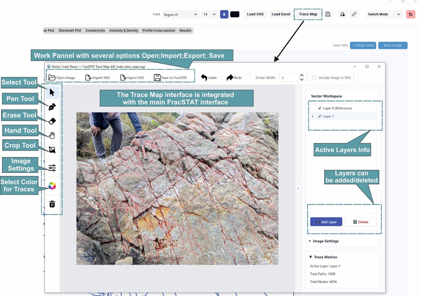
If all you have is a field photograph, use the integrated Trace Map tool to digitize fracture traces directly inside FracSTAT. The digitized traces feed straight into the same geometric, statistical and topological analysis as an imported SVG or Excel file — there is no need for external digitizing software.

Figure 2.4 — Data import using the "Trace Map" tab. Users select and upload a photograph, then digitize fracture traces using the fully integrated tool.

2. Digitizing with the Trace Map Tool

The Trace Map tool is a self‑contained digitization environment for converting field photographs of fractured outcrops into vector fracture maps. It is especially useful when you only have an outcrop photograph or scanned geological image and nothing already in digital form.

2.1 Top toolbar

Control	What it does
Open Image	Opens the field photograph or scanned image that will act as the digitizing reference.
Import SVG	Imports previously digitized traces (SVG) for further editing or refinement.
Export SVG	Exports the traced fracture network as a standard SVG file, for use in other vector/GIS software.
Save to FracSTAT	Saves the digitized network directly into the active FracSTAT project for analysis.
Undo / Redo	Reverses or restores the last editing operations.
Stroke Width	Adjusts the visual thickness of the digitized traces.
Include Image in SVG	Optionally embeds the reference image inside the exported SVG file.

2.2 Left‑hand tool palette

Tool	What it does
Select Tool	Selects existing traces for editing, repositioning, or deletion.
Pen Tool	The primary digitizing tool — manually trace fracture segments over the reference image, following each fracture as faithfully as possible.
Erase Tool	Removes unwanted traces or portions of existing digitized features.
Hand Tool	Pans across the workspace — useful for large outcrop images.
Crop Tool	Crops the reference image to the region of interest, improving mapping efficiency.
Image Settings	Adjusts brightness, contrast, or transparency of the reference image so traces are easier to see in different lighting.
Trace Colour	Assigns colours to traces — handy for distinguishing fracture sets, generations, lithological domains, or interpreters.

3. Calibrating the Scale

Once digitizing is finished, the traces are still in raw pixel space — they need a real‑world scale before any quantitative analysis means anything. Click the scale‑bar icon in the top‑right corner of the interface to open the Scale Calibration tool.

Figure 2.5 — Scale Calibration interface used to scale the fracture traces digitized from an outcrop image.

Figure 2.6 — Scale Calibration interface showing the function of the different tabs used to scale the digitized traces.

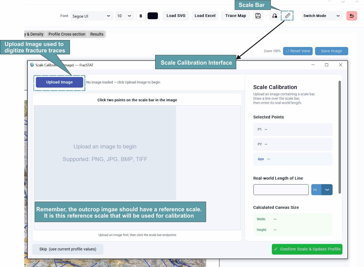
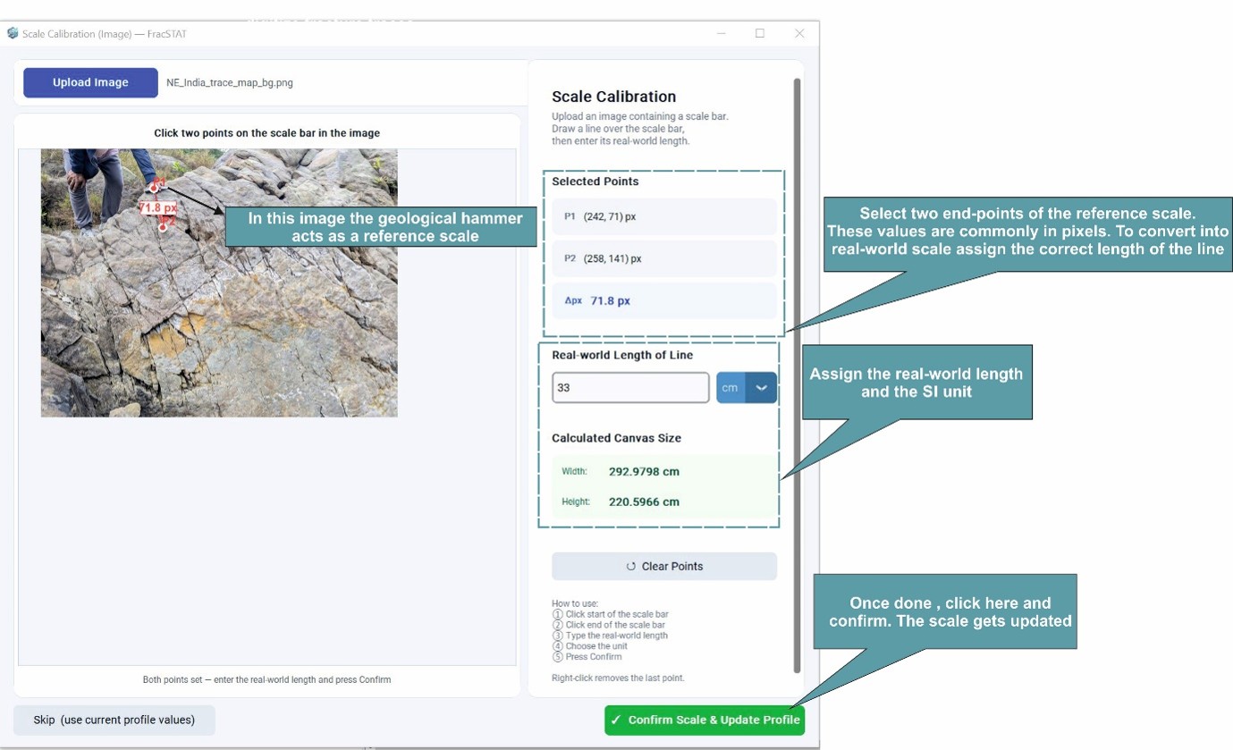
For SVG‑sourced data, raw digitizer coordinates (in pixel units) are rescaled into real‑world units by a single isotropic factor, taken from the calibration's units‑per‑pixel value where one exists and otherwise from an aspect‑preserving fit inside the physical profile box defined by the Profile Width and Profile Length fields (see Section 5.2). Because the same factor is applied to both axes, the traces may not fill the profile box exactly; angles and relative lengths are preserved instead. For spatial Excel/CSV data, no rescaling is performed — the coordinates are trusted to already be in real‑world units. The exact formulas are given in Section 8.

4. Fracture Map Interface Overview

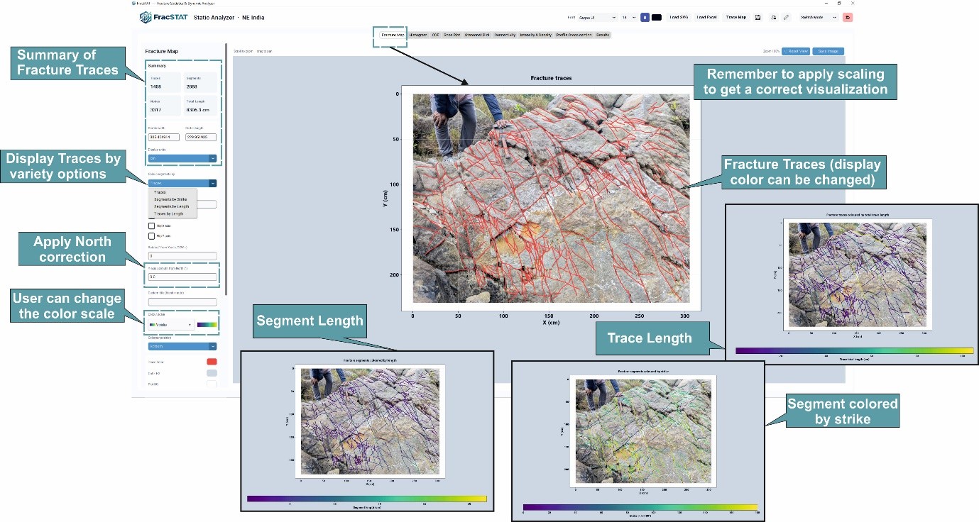
Once fracture traces have been imported (SVG), loaded (Excel), or digitized (Trace Map), they appear in the Fracture Map interface for inspection, editing, and quality control before any quantitative analysis runs. The tab is organised into three regions:

Region	Location	Description
Control Sidebar	Left panel (~290 px)	A scrollable column of cards containing every display setting, colour option, overlay toggle, and export control.
Map Canvas	Centre (resizable)	The primary Matplotlib canvas. Shows the fracture network, optional background photo, scale/units, and title.
Toolbar & Status	Top and bottom of the canvas	Shows pan/zoom hints, the current zoom percentage, and buttons to reset the view or save the current figure as an image.

Figure 2.7 — Fracture Map interface showing the spatial layout of digitized fracture traces on an outcrop image.

5. Sidebar Controls, Section by Section

The sidebar is organised top‑to‑bottom into collapsible cards. Each is explained below in the order it appears.

5.1 Summary

Four tiles give an at‑a‑glance overview of the loaded network, automatically recomputed every time the data or the profile changes:

• Traces — total number of distinct fracture traces (unique Trace IDs).
• Segments — total number of individual fracture segments (a trace may consist of several segments).
• Nodes — total count of topological nodes (I + Y + X + C — see Section 9).
• Total Length — sum of every segment's length, shown in your chosen display unit.

5.2 Profile & Units

Profile width and Profile length define the physical size (in the X and Y directions respectively) that the imported pixel geometry is rescaled to. Before any scale calibration is performed, these fields default to 260 m (Width) × 100 m (Length). Changing either value and pressing Enter re‑runs the geometry calculation and refreshes every tab. Display units lets you switch between metres, centimetres, millimetres and kilometres — FracSTAT automatically converts the profile width/length values for you when you change the unit, and keeps the Dynamic Analyzer workspace in sync.

These two fields set the box the geometry is fitted into, not the exact extent it is stretched to. Scaling is isotropic (Section 8.1), so only the more restrictive of the two limits binds and the traces may fall short of the other. If the mapped traces look smaller than the box you declared, that is aspect preservation doing its job — the alternative would silently shear every strike in the dataset. Where an exact units‑per‑pixel calibration exists, it takes precedence over these fields entirely.

5.3 Display Mode

Control	What it does
Colour segments by	Chooses how fracture lines are coloured — Traces, Segments by Strike, Segments by Length, or Traces by Length. See Section 6 for full detail.
Line width	Sets the rendered stroke width of every fracture line, in points.
Show segment nodes	Overlays a small marker at every segment endpoint (and at every calculated crossing point), useful for visually checking topology.
Show labels	Displays a text label on the map for each fracture segment, useful for cross‑referencing individual traces against a table or report.
Flip X axis / Flip Y axis	Mirrors the map horizontally or vertically — handy if your source image was scanned or photographed with an unexpected orientation.
Rotate (° from X axis, CCW+)	Rotates the whole map counter‑clockwise by the given number of degrees.
Y‑axis azimuth from North (°)	Tells FracSTAT how the image's vertical (Y) axis relates to true geographic north, so strikes reported everywhere in the software are north‑referenced rather than image‑referenced. See Section 8.2.

5.4 Plot Options

Control	What it does
Custom title	Overrides the automatic title (e.g. "Fracture segments coloured by strike") with your own text. Leave blank for the automatic title.
Colour scale	Chooses the colormap used whenever a continuous colour mode is active (Viridis, Plasma, Inferno, Parula, and more). A live swatch preview is shown next to the dropdown.
Colorbar position	Places the colour bar at the Bottom, Top, Left, or Right of the map, or hides it entirely ("None").

5.5 Map Elements

Fine‑tune the cosmetics of the figure without touching the underlying geometry:

Control	What it does
Trace Color	The single colour used when "Colour segments by" is set to Traces.
Outer BG	Background colour of the figure outside the plot area.
Plot BG	Background colour inside the plot axes.
Grid Color / Show grid lines	Colour and visibility of the coordinate grid behind the traces.
Show scale	Toggles a data‑accurate scale bar in the lower‑right of the map, drawn in the current display unit. The bar can be repositioned by dragging it directly on the map.
Scale Color	Colour used to draw the scale bar (and its label/ticks).
Scale style	Chooses how the scale bar is rendered — Solid bar (single filled block), Segmented bar (alternating filled/unfilled blocks), or Ticked line (a plain line with end ticks).
Border Color / Border Width	Colour and thickness of the axes border (spines).

5.6 Background Image

Enable Show real photo behind traces to draw your calibrated field photograph or orthophoto underneath the fracture lines — a quick visual sanity check that the traces line up with the real outcrop. Use Change Image… to pick a different photo, and Image opacity (0–1) to fade it so the traces stay legible on top. FracSTAT will try to auto‑detect a suitable image first (one you previously picked, a sidecar image saved next to a traced SVG, or one already calibrated in the Dynamic Analyzer workspace) before prompting you to browse for one.

5.7 Toolbar (above the canvas)

• ↺ Reset View — returns the map to its original zoom/pan position.
• Save Image — exports the current figure as a PNG at your configured export DPI.
• Zoom label — shows the current zoom percentage relative to the home view.

6. Colour Modes Explained

Mode	What is coloured	Best for
Traces	Every segment drawn in a single, user‑chosen colour (the "Trace Color" swatch).	Clean, simple maps and quick visual QC of trace geometry.
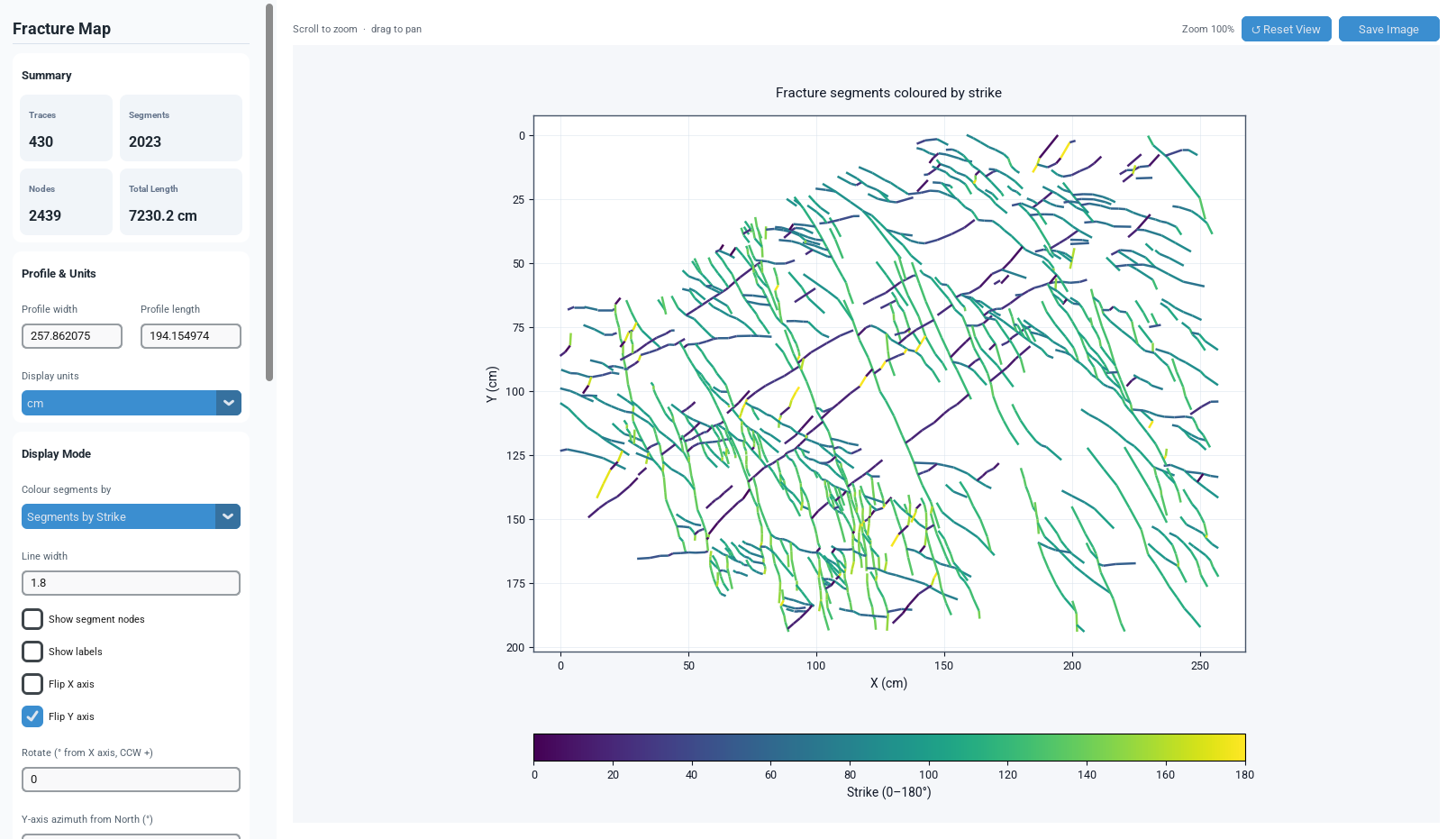
Segments by Strike	Each segment coloured by its strike, folded to the 0–180° convention (a fracture and its 180°‑reversed direction look the same, since traces are undirected lines).	Spotting dominant fracture sets and orientation trends at a glance.
Segments by Length	Each individual segment coloured on a linear scale from the shortest to the longest segment length.	Identifying short‑segment artefacts vs. genuinely long, continuous fractures.
Traces by Length	Every segment belonging to the same trace shares one colour, based on that trace's total length (all its segments summed together).	Understanding the true, full length of each fracture rather than its individual pieces.

Whenever a continuous colour mode is active, a colour bar is automatically added at the position chosen in Plot Options → Colorbar position, labelled with the plotted quantity and its units.

7. Zooming, Panning and Resetting the View

• Zoom — scroll the mouse wheel over the map. Zooming is centred on the cursor position, so whatever you're pointing at stays in view.
• Pan — click and drag anywhere on the map with the left mouse button.
• Reset — click ↺ Reset View in the toolbar to return to the original, fully‑zoomed‑out view.

Style changes (colour mode, colours, line width) preserve your current pan/zoom position, so you can zoom into an area of interest and try different display options without losing your place. Changes that alter the geometry itself — flipping an axis or rotating the map — reset the view, since the old zoom position no longer corresponds to the same part of the map.

8. The Maths Behind the Map

This section explains, in plain terms, exactly how FracSTAT turns raw digitized coordinates into the calibrated, north‑referenced map you see on screen.

8.1 Pixel‑to‑real‑world scaling (SVG data)

For SVG‑sourced data, raw digitizer coordinates (x, y), in SVG pixel units, are rescaled into real‑world units by a single isotropic factor applied to both axes. The factor is chosen by a three‑way rule, in this order:

Each endpoint is then transformed as:

The preferred branch is the middle one: the calibration dialog measures how many real‑world units one source pixel represents (units_per_px, computed in core/scale.py), and using it directly is both isotropic and exact, with no dependence on how much of the frame the traced fractures happen to cover. The min(…) fallback fits the trace bounding box inside the declared W × L profile rectangle while preserving aspect; because the calibration dialog derives W and L from a single px‑per‑unit value, W/L already equals the source pixel aspect ratio, so this recovers the true units‑per‑pixel when the traces span the calibrated frame and never introduces shear when they do not.

For spatial Excel/CSV data, no rescaling is performed — the coordinates are used at 1:1 physical scale, on the assumption that they already represent real‑world engineering or geographic units.

8.2 Strike (orientation) calculation

Field photographs aren't always taken with geographic north pointing to the top of the image. The Y‑axis azimuth from North setting corrects for this before any orientation‑based analysis (rose diagrams, stereographic projections) runs. Segment strike is first derived from the geometric orientation of its two rescaled endpoints. Because screen/SVG coordinates conventionally increase downward, the vertical delta is optionally inverted according to the "Reverse Y" setting:

This image‑referenced strike is then rotated into a north‑referenced strike using the Y‑axis azimuth from North (θₙ):

8.3 Segment length

Each segment's length is the Euclidean distance between its rescaled endpoints:

8.4 Trace length

A trace length is the sum of the lengths of every segment sharing the same Trace identifier — computed as a group‑by‑sum aggregation and joined back onto the segment table. This value feeds both the "Traces by Length" colour mode on this tab and the Histogram tab's trace‑length distribution and the Results tab's summary statistics.

8.5 Rotation

Applying the "Rotate" control spins every rescaled coordinate about the origin by the chosen angle θ (counter‑clockwise positive):

9. Fracture Topology & Node Counts

Every time the geometry is recalculated, FracSTAT looks at how many segment endpoints coincide at (roughly) the same point, and classifies each coincidence into a node type. These counts feed the "Nodes" summary tile and the "Show segment nodes" overlay, and describe how well‑connected your fracture network is. The node vocabulary is the standard fracture-network one (Sanderson and Nixon, 2015; Peacock et al., 2016).

Node type	How many segment ends meet there	Geological meaning
I‑node (isolated)	1	A free‑standing fracture tip that doesn't touch any other fracture — an isolated or under‑sampled end.
C‑node (continuation)	2	A simple joint between two segments — usually just a continuation point along a single digitized trace.
Y‑node (abutting)	3	One fracture terminates against another (a T‑junction) — the terminating fracture is typically younger than, or arrested by, the host fracture.
X‑node (crossing)	4 or more	Two (or more) fractures cross each other — suggesting they were active simultaneously, or sequentially with no mutual arrest.

The ratio of I : Y : X nodes is one of the best single indicators of network connectivity: a network dominated by I‑nodes has low connectivity (fluid flow would be limited and tortuous), while one dominated by Y and X nodes is highly connected (numerous, well‑linked flow pathways) (Sanderson and Nixon, 2015; Sanderson and Nixon, 2018). This ratio is explored further, and plotted, on the Connectivity tab.

10. Reading the Map Geologically

A well‑rendered fracture map encodes a lot of geological information. Work through these observations roughly in order:

10.1 Spatial distribution & clustering

A uniform scatter of fractures across the area suggests a pervasive, formation‑scale network. Clustering into corridors or bands can indicate proximity to faults, fold hinges, or lithological heterogeneities.

10.2 Fracture sets & cross‑cutting relationships

Switch "Colour segments by" to Segments by Strike to instantly see how many distinct orientation sets are present, and their relative proportions. Where traces cross (X‑nodes), the fracture that is cut by another is generally the older of the two (assuming they aren't exactly coeval). Where a trace abuts another (Y‑nodes), the terminating fracture is younger than, or coeval with, the fracture it grew into (Peacock et al., 2016).

10.3 Length distributions & sampling bias

Switching to Segments by Length or Traces by Length highlights two common biases: truncation bias (an excess of very short fractures relative to a true power‑law distribution — often a digitizing artefact) and censoring bias (traces whose true ends lie outside the mapped/scanned area) (Pickering et al., 1995; Bonnet et al., 2001). Traces whose endpoints lie fully inside the mapped area are "complete"; traces crossing the boundary are "censored". The balance between the two matters a great deal for the reliability of length‑distribution statistics in the Histogram and CDF tabs, and is also sensitive to the sampling scheme itself (Zeeb et al., 2013; Watkins et al., 2015).

10.4 Network connectivity

Check the I : Y : X node ratio (Section 9) — an I‑dominated network (e.g. 0.7 : 0.2 : 0.1) implies poor connectivity, while a Y/X‑dominated network (e.g. 0.1 : 0.4 : 0.5) implies a highly connected, well‑linked flow network (Sanderson and Nixon, 2018). The Connectivity tab visualises this on a standard ternary diagram.

11. Exporting a Figure

Click Save Image in the toolbar to export the current view of the map exactly as displayed. The image is saved as a PNG at the DPI configured in your app‑wide export settings (default 300 DPI), inside a per‑project export folder, and a confirmation dialog shows you the full file path once it's done.

12. Limitations

Limitation	Description
Resolution truncation	Very short fractures, below the digitizing pixel resolution, are systematically missed or over‑represented as noise, which truncates the low end of any length distribution fitted downstream (Pickering et al., 1995).
Profile box is a bound, not an extent	Because scaling is isotropic (Section 8.1), uncalibrated data is fitted inside the Profile Width × Length box rather than stretched to fill it, and one axis will generally have unused margin. The absolute scale of uncalibrated SVG data is therefore only as good as those two numbers; a genuine units‑per‑pixel calibration is the only route to an absolutely correct scale.
Map node tile is segment‑level	The Nodes summary tile and the "Show segment nodes" overlay classify coincident segment ends on a 0.01‑unit snap grid and include a C (continuation) class, so their counts depend on how finely traces were digitised and will not equal the Connectivity tab's trace‑level I/Y/X census (Section 9). Report the trace‑level census (Sanderson and Nixon, 2015) rather than this tile.
No orientation‑bias weighting on the map itself	Strike values are plotted as measured; the map applies no Terzaghi correction for fracture sets oriented unfavourably relative to the exposure or scanline direction (Terzaghi, 1965). Orientation‑unbiased intensity is estimated with circular windows on the Intensity & Density and Profile tabs (Mauldon et al., 2001).

13. Step‑by‑Step Example Workflow

Goal: produce a clean fracture map coloured by strike, calibrated to real‑world units, ready to export.

1. Open your project and go to the Fracture Map tab.
2. Import data using Load SVG, Load Excel, or digitize a photo with the Trace Map tool.
3. If prompted, complete the Scale Calibration step so the Profile Width/Length fields reflect real‑world dimensions.
4. In Profile & Units, confirm the width, length and display unit are correct.
5. In Display Mode, set "Colour segments by" to Segments by Strike, and set the correct Y‑axis azimuth from North.
6. In Plot Options, pick a colour scale (e.g. Viridis) and set the colour bar position.
7. In Map Elements, adjust background/grid/border colours to taste.
8. Zoom/pan to frame the area you want, then click Save Image in the toolbar.

14. Advanced & Related Capabilities

Beyond the core drawing pipeline described above, the Static Map Tab shares its underlying geometry, scale, and node‑topology data with the rest of FracSTAT's Static Module, so nothing computed here is wasted:

• Histogram & CDF tabs reuse the segment and trace length values computed on this tab.
• Rose & Stereonet tabs reuse the north‑corrected strike values computed here.
• Connectivity tab reuses the I/Y/X/C node counts to build ternary connectivity diagrams.
• Intensity & Density tab uses the same calibrated coordinate system to compute areal and linear fracture intensity (P21/P10/P20).
• Results tab presents the full per‑segment table (ID, Trace, Segment, coordinates, strike, dip, length, aperture) generated on this tab.

Switching to the Dynamic Analyzer workspace automatically carries your profile width/length, unit, and any calibrated background image across, so you don't have to recalibrate a second time.

15. References

Sources are listed alphabetically within each group. In-text citations throughout this page link to the corresponding entry below.

15.1 Fracture Mapping, Topology and Sampling

• Mauldon, M., Dunne, W. M., & Rohrbaugh, M. B. (2001). Circular scanlines and circular windows: new tools for characterizing the geometry of fracture traces. Journal of Structural Geology, 23(2–3), 247–258. https://doi.org/10.1016/S0191-8141(00)00094-8
• Peacock, D. C. P., Nixon, C. W., Rotevatn, A., Sanderson, D. J., & Zuluaga, L. F. (2016). Glossary of fault and other fracture networks. Journal of Structural Geology, 92, 12–29. https://doi.org/10.1016/j.jsg.2016.09.008
• Priest, S. D. (1993). Discontinuity Analysis for Rock Engineering. Chapman & Hall, London. https://doi.org/10.1007/978-94-011-1498-1 (Ch. 3: orientation measurement and projection.)
• Sanderson, D. J., & Nixon, C. W. (2015). The use of topology in fracture network characterization. Journal of Structural Geology, 72, 55–66. https://doi.org/10.1016/j.jsg.2015.01.005
• Sanderson, D. J., & Nixon, C. W. (2018). Topology, connectivity and percolation in fracture networks. Journal of Structural Geology, 115, 167–177. https://doi.org/10.1016/j.jsg.2018.07.011
• Terzaghi, R. D. (1965). Sources of error in joint surveys. Géotechnique, 15(3), 287–304. https://doi.org/10.1680/geot.1965.15.3.287
• Watkins, H., Bond, C. E., Healy, D., & Butler, R. W. H. (2015). Appraisal of fracture sampling methods and a new workflow to characterise heterogeneous fracture networks at outcrop. Journal of Structural Geology, 72, 67–82. https://doi.org/10.1016/j.jsg.2015.02.001
• Zeeb, C., Gomez-Rivas, E., Bons, P. D., & Blum, P. (2013). Evaluation of sampling methods for fracture network characterization using outcrops. AAPG Bulletin, 97(9), 1545–1566. https://doi.org/10.1306/02131312042

15.2 Length Scaling and Truncation Bias

• Bonnet, E., Bour, O., Odling, N. E., Davy, P., Main, I., Cowie, P., & Berkowitz, B. (2001). Scaling of fracture systems in geological media. Reviews of Geophysics, 39(3), 347–383. https://doi.org/10.1029/1999RG000074
• Pickering, G., Bull, J. M., & Sanderson, D. J. (1995). Sampling power-law distributions. Tectonophysics, 248(1–2), 1–20. https://doi.org/10.1016/0040-1951(95)00030-Q (Truncation and censoring effects on fracture-length samples.)