Dynamic Map Tab
Located at dynamic_analyzer/tabs/dynamic_map_tab.py, the Map Tab (implemented as the
MapTab mixin class) is the primary spatial visualization component of the
Dynamic Analyzer workspace within FracSTAT. Whereas the Static Analyzer's
Fracture Map tab presents purely geometric information (trace geometry, segment length,
orientation), the Dynamic Analyzer's Map Tab overlays the mechanical response of each fracture
segment — its resolved slip tendency, dilation tendency, fracture susceptibility, or binary
critical-stress state — onto the same spatial or angular reference frame from which the segment
was digitized.
This module functions as the geometric and cartographic rendering engine for the
SlipTendencyApp workspace (dynamic_app.py). It receives a fully
populated pandas DataFrame of per-segment stress-resolution results (produced by
core.calculator.run_calculation) and renders it using one of three complementary
spatial representations, automatically selected according to the nature of the loaded dataset:
- A true-to-scale Cartesian map for SVG-digitized trace networks and for Excel/CSV datasets that carry genuine X–Y coordinate geometry;
- A synthetic unit-circle orientation wheel for legacy Excel/CSV fracture-plane tables (Strike/Dip only, with no real spatial position);
- A geographic longitude–latitude scatter map, with optional embedded beachball diagrams, for Global-CMT-style focal-mechanism datasets.
The module also provides the calibrated real-world photographic background overlay, interactive pan/zoom, cross-tab segment highlighting, a fully configurable appearance settings panel, and a Move-Elements layout editor that lets the user reposition the plot axes and colour bar for publication-quality figure export.
On this page
- 1. Position within the FracSTAT Architecture
- 2. Interface Overview
- 3. Data Input and Prerequisites
- 4. Settings and Controls
- 5. Mathematical Background
- 6. Algorithms
- 7. Internal Workflow
- 8. Statistical Methods & Colour-Bar Geometry
- 9. Visualization Components
- 10. Advanced Features
- 11. Performance Optimization
- 12. Practical Examples
- 13. Geological Interpretation
- 14. Implementation Notes
- 15. Limitations
- 16. References
1. Position within the FracSTAT Architecture
The Map Tab is one of six tabs assembled inside SlipTendencyApp
(dynamic_app.py), the others being Rose, Mohr, Stereonet, Table, and Method. All six
tabs share a single results DataFrame (self.results) that is recomputed whenever the
user presses Calculate, changes a stress or geometry parameter, or loads a new SVG/Excel file. The
Map Tab does not perform stress resolution itself; it is a pure consumer of the DataFrame produced
by core/calculator.py and, for SVG data, the trace geometry produced by
core/svg_loader.py and core/models.py.
1.1 Data Flow
core.svg_loader.read_svg_segments()orcore.excel_loader.read_excel_segments()parse the source file into a list ofSegmentobjects.core.calculator.run_calculation()resolves the stress tensor onto each segment, producing columns such asStrikeDeg,DipDeg,SigmaN,Tau,SlipTendency,SlipTendencyNorm,DilationTendency,FractureSusceptibility,FractureSusceptibilityNorm,CriticalStress,CriticalStressValue,CriticalFactor,CriticalState,CriticalStateValue,X1/Y1/X2/Y2,RawX1…RawY2,Lat,Lon,EventLabel,PlaneName,BeachballURL, and related fields.dynamic_app.pystores this table asself.resultsand callsrefresh_plots(), which in turn callsMapTab._draw_map().MapTab._draw_map()dispatches to one of four internal drawing routines depending on the data source and the geometry actually present, and renders the result onto a Matplotlib Figure embedded in the Qt window viaFigureCanvasTkAgg.- User interaction with the Map Tab (segment selection, pan/zoom, appearance changes) feeds back into shared application state (
selected_segment_id, view limits) that the Mohr, Stereonet, and Table tabs also read, enabling synchronized cross-tab highlighting.
2. Interface Overview
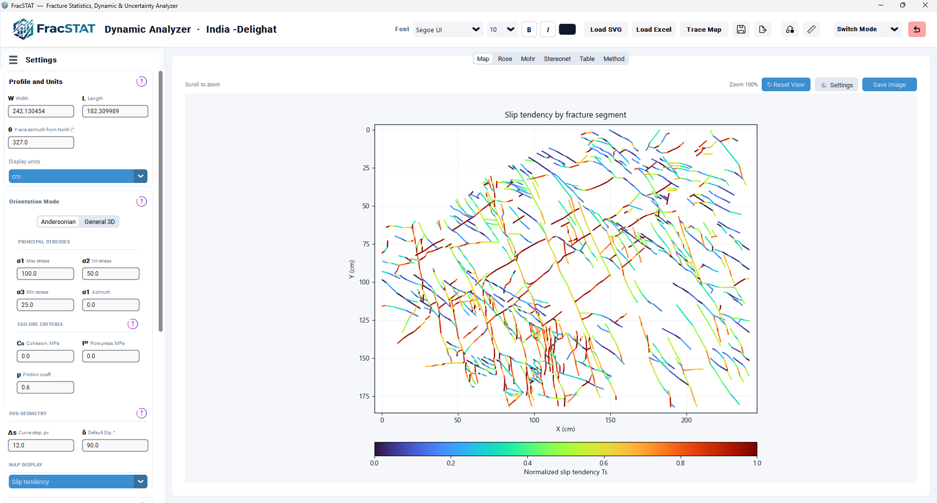
The Map Tab occupies the full content area of the "Map" tab within the Dynamic Analyzer's CTkTabview. Its layout is a two-column grid: a resizable plot area on the left (weighted to expand) and a collapsible settings panel on the right (fixed width, hidden by default).
2.1 Toolbar
A horizontal toolbar sits above the plot canvas and contains, from left to right:
| Control | Type | Function |
|---|---|---|
| "Scroll to zoom" label | Static label | Hint text reminding the user that the mouse scroll wheel zooms the plot. |
| Zoom percentage label | Dynamic label | Displays the current zoom level as a percentage of the home (fit-to-data) view, e.g. "Zoom 100%". |
| ↻ Reset View | Button | Restores the axis limits to the home view computed the last time the map was drawn from data. |
| ⚙ Settings | Toggle button | Shows or hides the appearance/settings panel on the right-hand side of the tab. |
| Save Image | Button | Exports the current figure (including any layout edits) to a PNG file in the project's plot-export folder, at the DPI configured in application settings. |
2.2 Plot Canvas
The plot canvas is a Matplotlib Figure (9 × 6 inches at 100 DPI) embedded via
FigureCanvasTkAgg, containing one primary Axes object (self.map_ax) for
the spatial or angular plot and one auxiliary Axes object (self.map_cbar_ax) reserved
for the colour bar. The canvas supports mouse-wheel zoom, click-and-drag pan (left button),
segment/event picking (for focal-mechanism data), and — when Move Elements mode is enabled from
the shared workspace header — direct dragging of the plot and colour-bar axes to arbitrary
positions within the figure.
2.3 Settings Panel
The settings panel is a CTkScrollableFrame, 230 px wide, that is not built into
the layout until the user first opens it via the ⚙ Settings toolbar button
(toggle_map_settings). It is organized into four labelled sections — Display
Options, Map Elements, Colour Bar, and Background Image — followed by a
Reset Map Defaults button. Every control in the panel is wired to immediately
redraw the map with preserve_view=True, so pan/zoom position is not lost while the
user experiments with appearance settings.
3. Data Input and Prerequisites
The Map Tab does not load files itself; it consumes state populated by the shared workspace
header's Load SVG / Load Excel actions and by core.calculator.run_calculation().
Three attributes on the parent SlipTendencyApp instance govern which drawing
routine is used:
| Attribute | Origin | Role |
|---|---|---|
self.results | core.calculator.run_calculation() | Per-segment DataFrame; the sole data source for every plotted element. |
self.data_source | "svg" or "excel" | Selected when a file is loaded; drives the top-level branch of the drawing dispatch. |
self.segments[0]._has_map_geometry | core.models.Segment | Boolean flag distinguishing genuinely spatial data (True) from orientation-only legacy fracture-plane or Trend/Plunge tables (False). |
3.1 Required and Optional Columns
Depending on the branch selected, the following results columns are read:
- Cartesian / SVG mode:
X1, Y1, X2, Y2(scaled, real-world units) andRawX1, RawY1, RawX2, RawY2(unscaled SVG pixel coordinates, used only when the profile has not yet been calibrated — see Section 5.3). - Orientation-wheel mode:
StrikeDeg,DipDeg,ID. - Geographic mode:
Lat,Lon,PlaneName,EventLabel,Region,BeachballURL. - All modes:
ID(for selection), plus whichever attribute column is selected for colouring (SlipTendency/SlipTendencyNorm,DilationTendency,FractureSusceptibility/FractureSusceptibilityNorm, orCriticalStateValue).
3.2 Coordinate Calibration Prerequisite
Cartesian rendering assumes the fracture network has been placed within a physically meaningful profile box. If the profile has not yet been calibrated (Width and Length sidebar fields still at their uncalibrated defaults of 260 and 100), the module falls back to plotting the raw, unscaled SVG pixel coordinates so that the original digitized proportions are preserved rather than being artificially stretched to fill a default 260 × 100 box — see the raw-coordinate detection logic described in Section 6.2.
4. Settings and Controls
This section documents every control in the Map Tab settings panel, its default value, its
valid range or accepted values, and its visual effect. All controls redraw the map immediately
upon change (preserve_view=True) except where noted.
4.1 Display Options
| Control | Widget | Default | Effect |
|---|---|---|---|
| Line width (SVG/Geo) | Text entry | 1.8 | Sets the LineCollection stroke width (points) for Cartesian traces, and separately scales the marker size of focal-mechanism event points (base_size = 85 × value) and orientation-wheel tick width. |
| Custom title (blank = auto) | Text entry | (empty) | Overrides the automatically generated plot title. When blank, a descriptive title is automatically generated based on the map mode (e.g., "Slip tendency by fracture segment" for Cartesian maps, "Slip tendency — fracture orientation wheel" for legacy Excel files, or "Slip tendency — focal mechanism map" for geographic data). |
| Show compass (Wheel Map) | Checkbox | On | Toggles the N/E/S/W compass labels drawn around the orientation wheel. Has no visible effect in Cartesian or geographic modes. |
Map Style (map_plot_style_var) | Dropdown | Fracture segments | Selects the surface rendering mode for Cartesian maps: Fracture segments (the default vector LineCollection rendering described in Section 6.2, no interpolation), Grid Heatmap (a Kriged/interpolated pcolormesh surface), Contour (Filled) (filled contour bands with optional line overlay), or Contour (Lines Only) (labelled contour lines with no fill). See Section 6.6. |
Contour Levels (map_contour_levels_var) | Text entry | 15 | Requested number of contour bands/lines when Map Style is one of the two contour modes; passed to _map_contour_levels() (Section 6.6). Reverts to 15 if the entered value cannot be parsed. |
Show fracture traces / points (map_show_traces_var) | Checkbox | On | Toggles whether the underlying fracture segments (or selection markers) are drawn on top of/underneath an interpolated surface. When Map Style is "Fracture segments" this is the only visible content; in surface modes it overlays the raw data on the Kriged surface for QC. |
Layer Order (map_layer_order_var) | Dropdown | Traces above surface | "Traces above surface" or "Surface above traces". Controls the stacking (z-order) of the fracture traces relative to the interpolated surface when both are shown together. |
Upper Layer Opacity (map_top_layer_opacity_var) | Slider | 0.8 (80%) | Alpha blending factor (10%–100%) applied to whichever layer — traces or surface — is currently on top, per the Layer Order setting, allowing the underlying layer to remain partially visible. |
Kriging Variogram Model (map_kriging_model_var) | Dropdown | linear | The variogram model passed to PyKrige's OrdinaryKriging: linear, power, gaussian, spherical, or exponential. Governs how spatial correlation is assumed to decay with distance during interpolation (Section 6.6). |
Grid Resolution (map_grid_resolution_var) | Text entry | 150 | Number of interpolation grid points per axis (valid range 30–400) used when computing the Kriged/interpolated surface. Higher values produce smoother surfaces at increased computation cost. |
Sample along segment length (map_segment_sampling_var) | Checkbox | On | When enabled, each fracture segment contributes three sample points (start, midpoint, end) to the interpolation input rather than just its midpoint, preventing long traces from collapsing to a single point and distorting the surface (Section 6.6). |
4.2 Map Elements
| Control | Widget | Default | Effect |
|---|---|---|---|
| Outer BG | Colour swatch | #F5F7FA | Figure (outer canvas) background colour. |
| Plot BG | Colour swatch | #FFFFFF | Axes (inner plot) background colour. |
| Grid Color | Colour swatch | #D9E2EC | Colour of the gridlines, when shown. |
| Show grid lines | Checkbox | On | Toggles the Matplotlib grid overlay. |
| Grid line width | Text entry | 0.6 | Line width (points) of gridlines; alpha is fixed internally at 0.6. |
| Boundary Color | Colour swatch | #1F2933 | Colour applied to all four Axes spines (the plot border). |
| Boundary width | Text entry | 1.0 | Line width (points) of the plot border spines. |
Show scale (map_show_scale_var) | Checkbox | Off | Toggles visibility of the data-accurate scale bar drawn in the map's lower-right corner by default (or wherever it has since been dragged to; see Section 10.1). |
Scale Color (map_scale_color_var) | Colour swatch | #1F2933 | Colour applied to the scale bar and its label text. |
Scale style (map_scale_style_var) | Dropdown | Solid bar | Rendering style of the scale bar: Solid bar, Segmented bar (alternating filled/unfilled segments), or Ticked line (a plain line with end and midpoint ticks). |
Contour Line Color (map_contour_line_color_var) | Colour swatch | #000000 | Stroke colour applied to contour line overlays, both in "Contour (Lines Only)" mode and for the optional line overlay drawn on top of "Contour (Filled)" surfaces. |
Contour Line Width (map_contour_line_width_var) | Text entry | 0.5 | Line width (points) of contour lines, clamped to a minimum of 0.1. |
4.3 Colour Bar
| Control | Widget | Default | Effect |
|---|---|---|---|
| Position | Dropdown | Bottom | Bottom / Top / Left / Right / None. Determines where the colour bar is docked and how the main Axes is resized to make room for it (see Section 8.4 for exact geometry). |
| Length (e.g., 0.8 for 80%) | Text entry | 1.0 | Fractional length of the colour bar relative to the corresponding figure dimension, clamped to [0.1, 1.0]. |
Force 0 to 1 scale (map_normalize_01_var) | Checkbox | Off | When enabled, forces the colour scale normalization to a strict [0.0, 1.0] range regardless of the attribute column's actual data range, overriding the empirical min/max behaviour described in Section 5.2. Useful for visually comparing surfaces or maps across different datasets on a common scale. |
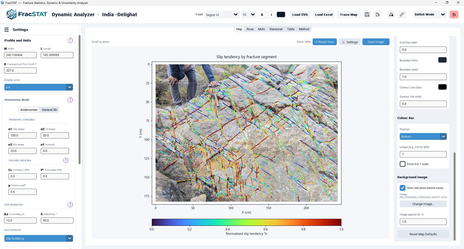
4.4 Background Image
| Control | Widget | Default | Effect |
|---|---|---|---|
| Show real photo behind traces | Checkbox | Off | Enables the calibrated background photograph overlay. If no image path is known, checking this box immediately opens a file-selection dialog; if the user cancels, the checkbox is reverted to off. |
| Status label | Read-only label | "No image set" | Displays the file name of the currently associated background image, or "No image set". |
| Change Image… | Button | — | Opens a file dialog (PNG/JPG/JPEG/BMP/TIFF/TIF/WEBP) to select or replace the background image; redraws immediately if the overlay is currently enabled. |
| Image opacity (0–1) | Text entry | 1.0 | Alpha blending factor applied to the background image via imshow, clamped to [0, 1]. |
4.5 Reset Map Defaults
The Reset Map Defaults button restores every Display Options, Map Elements, and
Colour Bar control to the factory values listed above and redraws the map with
preserve_view=True. By deliberate design, this reset does not clear the
Background Image settings (mode, path, or opacity): the code comment in the implementation notes
that "resetting plot cosmetics shouldn't silently detach a calibrated reference photo the user
deliberately attached." A calibrated photograph therefore survives a cosmetic reset and must be
removed explicitly by unchecking the Background Image checkbox.
5. Mathematical Background
5.1 Colour-Mapped Attributes
The Map Tab colours every plotted element (line segment, orientation tick, or event marker) according to one of four mechanical attributes, selected via the Display card's "Map Display" dropdown in the sidebar (outside the Map Tab itself, but consumed here) and the "Color by normalized Tₛ" checkbox. The mapping from the selected mode to a results column, axis label, and title fragment is:
| Map Display Mode | Normalized column | Raw column | Formula |
|---|---|---|---|
| Slip tendency | SlipTendencyNorm | SlipTendency | Tₛ = τ / σₙ |
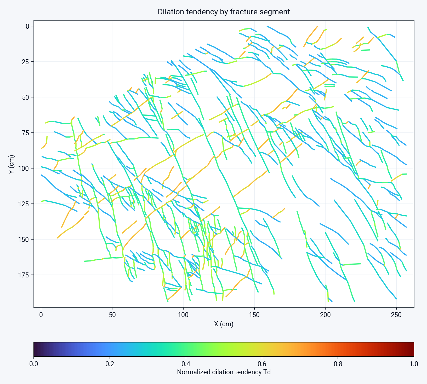
| Dilation tendency | — (always shown raw) | DilationTendency | T_d = (σ₁ − σₙ) / (σ₁ − σ₃) |
| Fracture susceptibility | FractureSusceptibilityNorm | FractureSusceptibility | S_f = σₙ − P_f − (τ − C₀) / μ |
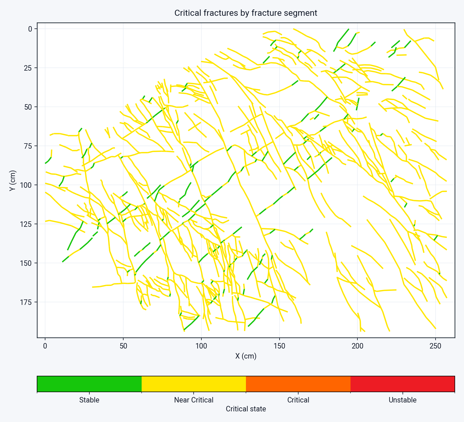
| Critical fractures | CriticalStateValue (four-tier) | — | 0 = Stable, 1 = Near Critical, 2 = Critical, 3 = Unstable, banded from threshold_ratio = [(τ − C₀) / (σₙ − P_f)] / μ at 50%/75%/100% |
5.1.1 Definition of Terms
- σₙ — normal stress resolved on the fracture plane (MPa), from the standard Cauchy stress transformation (Jaeger et al., 2007).
- τ — shear stress resolved on the fracture plane (MPa).
- σ₁, σ₃ — maximum and minimum principal stresses (MPa).
- P_f — pore-fluid pressure (MPa).
- C₀ — cohesion of the fracture surface (MPa).
- μ — coefficient of friction (dimensionless).
- Tₛ (Slip Tendency) — the ratio of resolved shear to normal stress; a plane slips when Tₛ approaches or exceeds μ (Morris et al., 1996).
- T_d (Dilation Tendency) — the propensity of a fracture to open (dilate) under the current stress state, normalized between the two principal stress extremes (Ferrill and Morris, 2003).
- S_f (Fracture Susceptibility) — a Mohr-Coulomb failure-margin proxy combining effective normal stress and cohesion-corrected shear stress; lower (more negative) values indicate closer proximity to shear failure, and the value is read most naturally as a tolerable pore-pressure increase (Streit and Hillis, 2004).
- threshold_ratio (Critical Fractures) — the friction coefficient required to resist the resolved shear stress, expressed as a fraction of the entered friction coefficient μ; see
core.calculator.critical_factor_and_state().
5.1.2 Normalization
When "Color by normalized Tₛ" is enabled, Slip Tendency is divided by a theoretical maximum
Tₛ,max computed analytically from σ₁ and σ₃ alone (independent of the sampled fracture set — see
core.calculator._theoretical_max_slip_tendency), guaranteeing that
which fractures happen to be present in the loaded dataset. FractureSusceptibilityNorm
is instead a min–max rescaling across the loaded fracture population, inverted:
1 − (S_f − S_f,min) / (S_f,max − S_f,min). The inversion matters for reading the map — because a
lower S_f means a smaller remaining pore-pressure margin, the least stable fractures are the ones
that map to 1.0 and therefore render at the "hot" end of the colormap; without it the colour
scale would run backwards. It also means S_f,norm is dataset-relative: 1.0 marks the least stable
fracture in the current file, not a fracture at failure, so normalized susceptibility maps should
not be compared between datasets (unlike SlipTendencyNorm, whose denominator is
theoretical). Where every fracture shares one S_f value the column collapses to 0.0 rather than
dividing by a zero range. Dilation Tendency is dimensionless by construction and
is never further normalized; Critical Fractures is likewise never rescaled, since its four
tiers are already fixed integer codes (0–3) rather than a continuous quantity.
5.2 Colour Normalization for Rendering
Once the attribute column is selected, MapTab.attribute_colormap_and_norm()
(delegating to SlipTendencyApp._attribute_norm in dynamic_app.py)
determines the Matplotlib Normalize object used to map data values to the 0–1
colormap domain:
- Columns ending in "Norm", plus
DilationTendency, use a fixedNormalize(vmin=0, vmax=1). - All other (raw, unnormalized) columns use the empirical minimum and maximum of the finite values present in the current dataset. If the data is degenerate (min ≈ max), a symmetric padding of 5% of the magnitude (or 1.0 if the value is exactly zero) is applied so the colour scale remains well-defined.
CriticalStateValueis treated specially: rather than a continuous colormap, a discrete four-colour colormap/norm is used so that the integer codes 0–3 (Stable, Near Critical, Critical, Unstable) are rendered as crisp, discrete bands rather than a misleading continuous gradient. The colour bar in this mode is relabelled with the ticks "Stable", "Near Critical", "Critical", and "Unstable" instead of numeric values. (The older binaryCriticalStressValuecolumn still exists in the results table for backward compatibility, but the Critical Fractures display mode no longer uses it.)
5.3 Cartesian Coordinate Scaling
For SVG-sourced traces, real-world segment endpoints (X1, Y1, X2, Y2) are computed upstream by
scaling the raw pixel bounding box of the digitized traces onto the user-specified Profile Width
× Profile Length box. Because the module cannot know from the DataFrame alone whether this
calibration has actually been performed, it applies a heuristic: if the scaled data's X-span and
Y-span are numerically close (relative tolerance 1 × 10⁻³) to the un-calibrated default profile
dimensions of 260 and 100 (the StringVar defaults for profile_width_var and
profile_height_var in dynamic_app.py), the module infers that no real
calibration has occurred and instead renders the RawX1/RawY1/RawX2/RawY2 pixel
columns, preserving the original digitized aspect ratio rather than an arbitrary default
stretch. Axis labels switch accordingly from "X (unit)"/"Y (unit)" to "X (px)"/"Y (px)".
5.4 Orientation-Wheel Geometry
For legacy Excel/CSV fracture-plane tables with Strike/Dip but no spatial coordinates, each fracture is represented as a short radial tick mark on a unit circle (radius R = 1). Let θ be the strike azimuth in radians (compass convention: 0° = north, increasing clockwise) and δ be the true dip in degrees. The tick's centre point is:
and the tick extends symmetrically along the local perpendicular direction, (cos θ, −sin θ), by a half-length of:
so that a vertical fracture (δ = 90°) is drawn as the longest possible tick, while a horizontal (bedding-parallel, δ = 0°) fracture collapses to a point — an intuitive visual analogue of true dip magnitude. The wheel therefore encodes strike as angular position around the circle and dip as radial tick length, giving a compact one-glance summary of the orientation population without requiring real spatial coordinates.
5.5 Geographic (Focal-Mechanism) Projection
For focal-mechanism datasets, event locations are plotted directly in longitude/latitude space. Because one degree of longitude does not span the same physical distance as one degree of latitude away from the equator, the Axes aspect ratio is corrected by:
where latitude_mean is the arithmetic mean latitude of the plotted events. This keeps circular/point features visually undistorted at the map's characteristic latitude, using a lower bound of 0.15 to avoid an unbounded aspect ratio near the poles. It is a local aspect correction, not a true cartographic projection (Snyder, 1987), so distances and areas should not be measured off the plotted axes.
5.6 Interactive Zoom Mathematics
Mouse-wheel zooming is implemented as a cursor-anchored rescaling of the current axis limits. Given a zoom factor f (0.85 per "scroll up" step, 1.18 per "scroll down" step) and cursor data-coordinates (cx, cy), the fractional position of the cursor within the current view is computed for each axis, e.g. for x:
The axis span is then scaled by f and the new limits are placed so that the cursor's fractional position within the view is preserved, i.e. the point under the cursor remains stationary on screen while the surrounding view expands or contracts. The same logic is applied independently to the y-axis, and correctly accounts for inverted axis directions (relevant when the SVG Y-axis convention places larger Y values toward the top of the screen).
6. Algorithms
6.1 Drawing Dispatch Algorithm
Every call to _draw_map() begins by determining which of four internal renderers
should handle the current dataset. The decision tree, implemented in _draw_map() and
mirrored in the table below, is evaluated in this priority order:
| Step | Condition Tested | Routine Invoked |
|---|---|---|
| 1 | data_source == "excel" and segments[0]._has_map_geometry is False | _draw_map_no_geometry — explanatory empty-state message |
| 2 | data_source == "excel", geometry present, and "Lat" column has at least one non-null value | _draw_map_geo — geographic focal-mechanism map |
| 3 | data_source == "excel", geometry present, no Lat data, and "Length" column is not uniformly zero | _draw_map_svg — Cartesian map using the genuine X/Y coordinates supplied by the spreadsheet |
| 4 | data_source == "excel", none of the above (legacy Strike/Dip table) | _draw_map_excel — synthetic orientation wheel |
| 5 | data_source == "svg" (default branch) | _draw_map_svg — Cartesian map from digitized trace geometry |
def _draw_map(self, preserve_view=False):
    if getattr(self, "data_source", "svg") == "excel":
        segs = getattr(self, "segments", None)
        has_geometry = bool(segs) and getattr(segs[0], "_has_map_geometry", True)

        # 0. No real spatial coordinates and no Lat/Lon — e.g. a legacy
        #    fracture-plane file or a Trend/Plunge pole file. There is no
        #    meaningful map to draw, so show an explanatory empty state.
        if not has_geometry:
            self._draw_map_no_geometry(preserve_view)

        # 1. Geographic Data (Focal Mechanisms)
        elif "Lat" in self.results.columns and self.results["Lat"].notna().any():
            self._draw_map_geo(preserve_view)

        # 2. Raw Coordinate Data (Spatial Map)
        elif "Length" in self.results.columns and not (self.results["Length"] == 0).all():
            self._draw_map_svg(preserve_view)

        # 3. Legacy Strike/Dip (Orientation Wheel)
        else:
            self._draw_map_excel(preserve_view)
    else:
        # Standard SVG
        self._draw_map_svg(preserve_view)
Simplified excerpt of the drawing dispatch logic implemented in _draw_map().
6.2 Cartesian Rendering Algorithm (_draw_map_svg)
- Preserve the current axis limits if
preserve_viewis requested and a home view already exists. - Clear the plot and colour-bar Axes and apply the outer/inner background colours.
- Determine whether raw (uncalibrated) or scaled coordinates should be used, per the heuristic in Section 5.3.
- Reshape the endpoint columns into an (N, 2, 2) array suitable for a Matplotlib
LineCollection. - Compute the data bounding box and draw the calibrated background photograph, if enabled, beneath the traces (zorder = 0).
- Apply a 2% padding margin to the bounding box so that boundary segments are not visually clipped.
- Resolve the active colouring attribute and its colormap/normalization (Sections 5.1–5.2), build the
LineCollectionwith per-segment colour values, and add it to the Axes. - If a segment is currently selected (
selected_segment_id), redraw it with a two-layer halo-and-core highlight (a thick under-stroke in the text colour, a slightly narrower over-stroke in the failure/accent colour) plus endpoint markers, so the selection remains visible against any colormap. - Position and populate the colour bar according to the chosen dock position (Section 5.4), or hide it and expand the plot Axes if "None" is selected.
- Apply axis limits (respecting the Y-axis reversal setting), then set the aspect ratio to 'equal' with
adjustable='box'— deliberately applied after the limits so the plot area shrinks to fit the data rather than stretching the data to fill the plot area. - Store the resulting (pre-aspect-correction) tight data bounds as the new "home" view for the Reset View button and zoom-percentage calculation.
- Apply axis labels, title, gridlines, and boundary spine styling; refresh the zoom label; request an idle canvas redraw.
6.3 Orientation-Wheel Rendering Algorithm (_draw_map_excel)
- Draw the unit-circle boundary ring and, if enabled, the four compass labels.
- For each fracture, compute its tick centre and half-length per Section 5.4, colour it by the active attribute, and collect all ticks into a single
LineCollectionfor efficient rendering. - If a segment is selected, recompute its tick position and draw the same halo-and-core highlight pattern used in Cartesian mode, plus an "ID n" text annotation offset from the tick.
- Fix the axis limits to a symmetric [-1.35, 1.35] box (turning off axis ticks and labels, since the wheel has no physical coordinate system), apply the descriptive title, and finalize styling exactly as in Cartesian mode.
6.4 Geographic Rendering Algorithm (_draw_map_geo)
- Reduce the results table to one representative row per event: rows tagged
PlaneName == "FP1"are preferred when present (so two-nodal-plane focal mechanisms are not double-plotted); otherwise rows are de-duplicated on the (Lat, Lon) pair. - Resolve the active attribute for colouring and build a single scatter plot of all events, with marker size proportional to the Line width control.
- Compute padded longitude/latitude limits (12% of the data range, or a fixed 0.5–1.0° minimum pad for single-point or degenerate datasets) and apply the latitude-corrected aspect ratio from Section 5.5.
- If a segment/event is selected, draw a double concentric-ring highlight around it, an event-label annotation, and — if a Beachball URL is present for that event — invoke the beachball inset renderer (Section 9.2).
- Position the colour bar and finalize styling as in the other two modes.
6.5 Empty-State Algorithm (_draw_map_no_geometry)
When the loaded Excel/CSV table has neither spatial coordinates nor latitude/longitude columns (e.g. a legacy fracture-plane file lacking even orientation-wheel-compatible fields, or a Trend/Plunge pole file), the module deliberately avoids drawing a misleading synthetic map. Instead it clears the Axes, hides the colour bar, and displays a centred, word-wrapped explanatory message directing the user to the Table, Rose, Mohr, and Stereonet tabs, where orientation and stress results remain fully available.
6.6 Kriging & Surface Interpolation Engine
When Map Style is set to Grid Heatmap or either Contour mode, the Cartesian renderer
(_draw_map_svg) delegates surface construction to _krige_map_surface()
rather than drawing the raw LineCollection alone. This engine interpolates the
selected attribute across a regular grid spanning the data bounding box, using the ordinary
kriging predictor and its underlying variogram model of spatial autocorrelation
(Cressie, 1993;
Chilès and Delfiner, 2012):
- Sample-point extraction — each fracture segment contributes one (midpoint-only) or three (start, midpoint, end — see below) spatial sample points, depending on the "Sample along segment length" setting, each tagged with the segment's value for the active colouring attribute.
- Cache lookup — a BLAKE2b hash is computed over the sample dataset, the selected value column, the spatial bounds, the chosen variogram model, and the grid resolution. If an identical hash is found in
self._map_krige_cache, the previously computed grid is reused immediately and no recomputation occurs — this makes toggling between Map Style options or cosmetic settings instantaneous after the first interpolation. - Asynchronous computation — on a cache miss,
_show_map_kriging_loader()displays a progress overlay on the plot canvas and the interpolation itself is dispatched to a background daemon thread, keeping the Qt main thread (and therefore the rest of the UI) responsive while the surface is computed. - Interpolation fallback chain — the engine first attempts
OrdinaryKrigingfrom the PyKrige library using the selected variogram model. If PyKrige is not installed, or the kriging system is singular for the current sample configuration (raising aLinAlgWarning), the engine falls back to SciPy'sgriddata(Virtanen et al., 2020), itself attempted in order of decreasing interpolation quality:cubic→linear→nearest, so that a surface is always produced even for degenerate or sparse sample sets. - Result caching and marshalling — once the background thread completes, the resulting grid is stored in
self._map_krige_cachekeyed by the hash computed in step 2, and the map is redrawn; the redraw call that triggered the original cache miss will, on completion, hit the now-populated cache.
6.6.1 Three-Point Segment Sampling
A naive interpolation input would sample each fracture segment only at its midpoint. For long traces this can misrepresent the spatial footprint of the fracture, effectively collapsing an extended linear feature into a single point during interpolation. When "Sample along segment length" is enabled, each segment instead contributes three points, parameterized along its length by t ∈ {0.0, 0.5, 1.0} (start, midpoint, end), all carrying the same attribute value. This more faithfully represents long traces spanning multiple grid cells and reduces artefacts where a long fracture would otherwise appear as an isolated data point in the interpolated surface.
6.7 Surface Rendering Algorithm (_draw_map_surface)
Once _krige_map_surface() has returned a grid, _draw_map_surface()
renders it according to the selected Map Style:
- Grid Heatmap — the interpolated grid is drawn with
pcolormesh, coloured by the active attribute's colormap and normalization (Sections 5.1–5.2). - Contour (Filled) — the grid is drawn with
contourfusing levels computed by_map_contour_levels(), optionally with a thincontourline overlay on top in the configured Contour Line Color/Width for band-boundary clarity. - Contour (Lines Only) — only
contouris called (no fill), with each line styled per the Contour Line Color/Width controls and directly labelled with its numerical value via Matplotlib's contour-label mechanism.
_map_contour_levels() determines the tick/level values passed to contourf/contour: it uses Matplotlib's MaxNLocator (or, when "Force 0 to 1 scale" is enabled, fixed interval steps across [0, 1]) to generate the requested number of levels (Contour Levels setting) spanning the surface's data-driven or forced min/max.
Finally, _show_map_colorbar() decides whether the colour bar is drawn at all for the current style: it is automatically suppressed in "Contour (Lines Only)" mode, since the contour lines are already individually labelled with their values and a colour bar would be redundant and add visual clutter; the colour bar is shown normally for Grid Heatmap, Contour (Filled), and the default Fracture segments style.
When both a surface and the fracture traces/points are shown (Show fracture traces / points enabled), the Layer Order and Upper Layer Opacity controls determine which is drawn on top and how transparent that top layer is, allowing the raw data to be cross-checked visually against the interpolated surface without one completely obscuring the other.
7. Internal Workflow
The Map Tab participates in the broader Dynamic Analyzer refresh cycle as follows:
- The user loads an SVG or Excel/CSV file, or edits a stress/geometry parameter, or clicks Calculate.
SlipTendencyApp.calculate()(dynamic_app.py) invokescore.calculator.run_calculation()and stores the returned DataFrame asself.results.SlipTendencyApp.refresh_plots()is called, which invokesMapTab._draw_map(preserve_view=...)alongside the Rose, Mohr, and Stereonet tabs' own redraw methods._draw_map()runs the dispatch algorithm of Section 6.1 and delegates to the appropriate renderer.- The renderer clears and repopulates the Matplotlib Axes, updates
self._map_home_limits, and callsdraw_idle()on theFigureCanvasTkAggfor an efficient, non-blocking repaint. - Subsequent user interactions — mouse-wheel zoom, click-drag pan, segment selection in this or another tab, or a settings-panel change — call
_draw_map(preserve_view=True)so the current pan/zoom state (rather than the freshly computed home view) is retained across cosmetic or selection-only updates.
7.1 Cross-Tab Segment Selection
Clicking a focal-mechanism event marker (geographic mode only; Cartesian and wheel modes do not
currently support direct click-to-select on the map itself) triggers on_map_pick(),
which resolves the picked scatter index back to a segment ID via the parallel
_map_geo_ids array and calls the shared select_segment() method on the
parent application. This, in turn, updates selected_segment_id and triggers a
synchronized redraw of the Map, Mohr, and Stereonet tabs, and refreshes the Table tab's active
row — so a fracture identified as critically stressed in the Mohr diagram can be located
instantly on the map, and vice versa.
7.2 State Persistence
Several pieces of Map Tab state persist across saves/reloads of a project session (see
core/project_state.py): the background-image mode flag, image path, and opacity are
written into the saved session JSON so a calibrated photograph reattaches automatically when the
project is reopened. Pan/zoom position and the settings-panel open/closed state are, by contrast,
session-local UI state and are not persisted.
8. Statistical Methods and Colour-Bar Geometry
8.1 Descriptive Range Handling
For raw (non-normalized) attribute columns, the module relies on the empirical minimum and
maximum of the finite values in the current results table (Section 5.2)
rather than any fixed theoretical range. This is a deliberate choice: because Fracture
Susceptibility and raw Slip Tendency have stress-tensor-dependent physical ranges, a fixed
colour scale would either clip informative variation or waste dynamic range on datasets with a
narrow spread. The 5% padding rule for degenerate (single-value) datasets prevents a
divide-by-zero condition in Matplotlib's Normalize and ensures the colour bar always
renders a visible, non-degenerate gradient.
8.2 Critical-Fracture Classification Display
The Critical Fractures mode is a four-class statistical summary rather than a continuous field:
each segment's threshold_ratio — the friction demand required to resist its
resolved shear stress, expressed as a fraction of the entered friction coefficient μ — is
banded into Stable (0–50%), Near Critical (50–75%), Critical (75–100%), or Unstable (>100%),
via core.calculator.critical_factor_and_state(). The Map Tab renders this
classification with a discrete four-colour palette and boundary-normalized colour mapping
(Section 5.2) so that the discrete nature of the result is never
misrepresented as a continuous gradient — a common source of misinterpretation in geomechanical
figures.
8.3 Event De-duplication (Geographic Mode)
Focal-mechanism datasets may contain one or two nodal-plane rows per physical earthquake. The Map Tab's de-duplication step (preferring the FP1-tagged row, or otherwise the first occurrence of each unique Lat/Lon pair) ensures that summary statistics implied by the map — the number of markers, their spatial density — correctly reflect the number of physical events rather than the number of nodal-plane table rows.
8.4 Colour-Bar Docking Geometry
The exact rectangle occupied by the colour bar Axes, and the corresponding resize of the main plot Axes, is computed from the user-selected Position and Length settings as follows (all values in figure-fraction coordinates; L = user-configured colour-bar length fraction):
| Position | Colour-bar rectangle (left, bottom, width, height) | Main-axes rectangle (left, bottom, width, height) |
|---|---|---|
| Bottom | (0.5 − L/2, 0.07, L, 0.03) | (0.08, 0.18, 0.88, 0.74) |
| Top | (0.5 − L/2, 0.92, L, 0.03) | (0.08, 0.06, 0.88, 0.78) |
| Left | (0.03, 0.5 − L/2, 0.02, L) | (0.12, 0.06, 0.84, 0.88) |
| Right | (0.94, 0.5 − L/2, 0.02, L) | (0.06, 0.06, 0.84, 0.88) |
| None | (colour bar hidden) | (0.08, 0.06, 0.88, 0.88) |
(Note: The exact fractional coordinates shown above reflect the Cartesian/SVG rendering mode. The Orientation Wheel and Geographic rendering modes utilize slightly adjusted docking rectangles to safely accommodate their unique radial and geographic axis labels.)
For Critical Fractures colouring, the colour bar's tick marks are overridden to display the text labels "Stable", "Near Critical", "Critical", and "Unstable" at positions 0–3, in place of numeric tick values.
9. Visualization Components
9.1 Line and Marker Rendering
All fracture segments (or orientation ticks) sharing a common colouring attribute are rendered
as a single Matplotlib LineCollection rather than as individually plotted lines.
This is both a performance optimization (Section 11) and a
visual-consistency measure, since a LineCollection guarantees uniform handling of
colour mapping, z-ordering, and anti-aliasing across the entire fracture population
(Hunter, 2007).
9.2 Beachball Diagram Insets
For focal-mechanism datasets that supply a Beachball URL, selecting an event renders an inset
diagram card near that event's marker using Matplotlib's offsetbox machinery
(AnnotationBbox, OffsetImage, VPacker,
DrawingArea, TextArea). The beachball itself is a lower-hemisphere
equal-area plot of the radiation pattern in the standard seismological convention
(Aki and Richards, 1980;
Dahlen and Tromp, 1998), retrieved as a pre-rendered
image rather than computed here. The inset card displays:
- A bold title line showing the event label (or "Focal mechanism" if unavailable);
- The downloaded beachball image, once available, rendered via
OffsetImage; - A live "Loading…" placeholder — a circular ring with a coloured arc segment mimicking a spinner — while the image is still downloading;
- An "Image unavailable" placeholder if the download failed.
The card is drawn with a rounded, semi-transparent background box, an arrow connector back to the event's map location, and (where the Matplotlib version supports it) a subtle drop-shadow path effect for visual depth, styled to match the current light/dark appearance mode.
9.3 Selection Highlighting
Across all three rendering modes, the currently selected fracture is emphasized with a consistent two-layer "halo and core" technique: a wider stroke in the workspace text colour is drawn first, followed by a narrower stroke in the failure/accent colour on top, producing a high-contrast outline that remains legible regardless of the underlying colormap. Endpoint or event markers are added in the accent colour with a contrasting edge, and — in geographic and wheel modes — a short text label identifying the segment ID or event label is annotated nearby.
9.4 Background Photograph Overlay
The calibrated real-world photograph, when enabled, is drawn beneath all vector content (zorder
= 0) using imshow with an extent tuple of (xmin, xmax, ymax, ymin) rather than the
more conventional (xmin, xmax, ymin, ymax). This intentional vertical flip compensates for the
SVG coordinate convention (Y increasing downward) so that the photograph aligns pixel-for-pixel
with the overlaid trace geometry rather than appearing upside-down relative to it.
10. Advanced Features
10.1 Move Elements Layout Editor
When Move Elements mode is enabled from the shared workspace header (top toolbar, outside this
module), clicking and dragging inside the map or colour-bar Axes repositions that Axes' bounding
box within the figure, in real time, by translating the mouse displacement in screen pixels into
figure-fraction coordinates. This allows the user to manually compose a publication-ready layout
— for example, shrinking the plot slightly and relocating the colour bar to an unconventional
position — before using Save Image to export a high-resolution figure. The Map Tab intercepts
these press/motion/release events itself (_on_layout_press,
_on_layout_motion, _on_layout_release) rather than relying solely on
the generic cross-tab layout-editing handlers used by the Rose, Mohr, and Stereonet tabs, because
the Map Tab's canvas also has ordinary pan/zoom bindings on the same mouse buttons that must be
suppressed while editing is active.
When the scale bar (Section 4.2) is visible, the same edit mode also lets the
user click and drag the scale bar itself (_map_scale_bar) to any position within the
map Axes, independently of the Axes-repositioning behaviour described above. On press, if the
cursor is inside the scale bar's current window extent, the handler begins tracking a scale-bar
drag instead of an Axes drag; on motion, the pixel displacement is converted to Axes-fraction
coordinates and applied to the bar via set_bbox_to_anchor, clamped to keep the bar
within the plot (x in [0.05, 1.0], y in [0.0, 1.0]); on release, the new position
(_map_scale_position) is retained so the bar reappears in the same spot after a
redraw, until Reset Map Defaults restores it to the default lower-right corner.
10.2 Calibrated Background Photograph Auto-Detection
The module attempts to automatically reattach a background photograph without requiring the user to re-browse for it, using a three-tier fallback search: (1) the path already stored for this session, if the file still exists; (2) a sidecar PNG file named after the source SVG ("<name>_bg.png"), automatically written by the Trace Map tool when a photograph was calibrated there; (3) a photograph already calibrated in the Static Analyzer workspace for the same project, shared live via the launcher's cross-workspace state. This means a single calibration performed anywhere in the application — the Trace Map tool, the Static Analyzer, or the Dynamic Analyzer's own Scale dialog — becomes available to the Map Tab without repetition.
10.3 Asynchronous Beachball Retrieval
Beachball diagram images are fetched over HTTP in a background ThreadPoolExecutor
(four worker threads) rather than on the Qt main thread, so downloading a diagram from an
external URL never freezes the user interface. Each URL is tracked in one of three sets —
cached (successfully loaded), pending (download in progress), or failed (download attempted and
unsuccessful) — and a completed download is marshalled back onto the main thread via the
Qt after() scheduling mechanism, which then triggers a targeted redraw of the
map only if the just-loaded image belongs to the currently selected event.
10.4 Reference-Image Prefetching
prefetch_beachballs() allows the calling code (invoked when an Excel
focal-mechanism file is first loaded) to warm the cache for every event's beachball URL in the
dataset up front, so that once the user begins clicking through events the corresponding
diagrams are already downloaded or in flight, minimizing perceived latency during interactive
exploration.
11. Performance Optimization
| Technique | Applied To | Benefit |
|---|---|---|
| Vectorized LineCollection / batched scatter | All fracture segments, orientation ticks, or focal-mechanism markers | A single collection object is added to the Axes per redraw instead of hundreds or thousands of individual plot() / scatter() calls, dramatically reducing Matplotlib artist-management overhead. |
draw_idle() instead of draw() | Every redraw path | Matplotlib defers the actual repaint to the next Qt event-loop idle slot and coalesces rapid successive redraw requests (e.g. during a drag), avoiding redundant repaints. |
| Background-image pixel cache | _load_bg_image_array via _bg_image_cache tuple (path, array) | The photograph is decoded from disk only once per unique path; repeated redraws (pan, zoom, cosmetic changes) reuse the cached NumPy array. |
| Threaded network I/O | Beachball image downloads | HTTP fetches (up to 8-second timeout each) run off the UI thread in a 4-worker pool, keeping the interface responsive while multiple diagrams load concurrently. |
preserve_view flag | All redraw call sites | Avoids unnecessarily recomputing and resetting the home view / axis limits on every cosmetic change, preserving the user's current pan/zoom position and avoiding a jarring view reset. |
BLAKE2b-keyed surface cache (_map_krige_cache) | Kriged/interpolated surfaces (Grid Heatmap, Contour styles) | Interpolation is only recomputed when the dataset, value column, spatial bounds, variogram model, or grid resolution actually change; toggling between Map Style options or unrelated cosmetic settings reuses the cached grid instantly. |
| Background-thread kriging | _krige_map_surface() | The (potentially expensive) interpolation computation runs on a daemon thread rather than the Qt main thread, so the UI remains responsive and a progress overlay can be shown while a new surface is computed. |
12. Practical Examples
12.1 Example 1 — Mapping Slip Tendency on a Digitized Fault Network
- Load a fracture-trace SVG via the workspace header's Load SVG button.
- Calibrate the profile scale (Scale button) against a known reference length in the source image.
- Enter appropriate principal stress magnitudes and orientation in the sidebar, then click Calculate.
- On the Map Tab, confirm the sidebar's Map Display mode is set to "Slip tendency" and "Color by normalized Tₛ" is checked.
- Segments rendered in the colour bar's upper range represent fractures whose resolved shear-to-normal stress ratio approaches the frictional threshold — the most mechanically favourable orientations for reactivation under the current stress state.
- Click a segment of interest in the Table tab to see it highlighted with the halo-and-core marker on the Map, and cross-check its exact Tₛ and Mohr-diagram position in the Mohr tab.
12.2 Example 2 — Visualizing a Legacy Fracture-Plane Spreadsheet
- Load an Excel/CSV file containing only ID, Strike, and Dip columns (no spatial coordinates).
- The Map Tab automatically falls back to the orientation-wheel renderer, since no genuine geometry is present.
- Set Map Display to "Fracture susceptibility" to visualize which orientations are closest to the Mohr-Coulomb failure envelope, independent of their (unknown) spatial position.
- Enable "Show compass (Wheel Map)" to retain the N/E/S/W frame of reference while interpreting tick azimuths as fracture strike.
12.3 Example 3 — Focal-Mechanism Regional Stress Screening
- Load a Global-CMT-style Excel file with Lat, Lon, FP1 Strike/Dip/Slip (and optionally FP2) columns.
- The Map Tab automatically renders a geographic scatter map; enter a candidate regional stress tensor and click Calculate.
- Set Map Display to "Critical fractures" to immediately identify which historical earthquakes are kinematically consistent with reactivation under the candidate stress field, ranked into four bands — Stable, Near Critical, Critical, and Unstable — rather than a simple yes/no split.
- Click an event marker to open its beachball diagram inset and inspect the Rake Misfit reported in the pole-inspector text panel alongside the resolved shear along the slip vector and the predicted rake (the same panel is shared by the Map, Mohr and Stereonet tabs; the misfit is labelled "consistent" at ≤ 30°). It quantifies how well the entered stress tensor explains that earthquake's observed slip direction.
13. Geological Interpretation
13.1 Slip Tendency Maps
Spatial or angular clusters of high slip tendency indicate structural elements that are mechanically well-oriented for frictional reactivation under the assumed stress field. In fault-reactivation risk assessment, induced-seismicity screening, and reservoir-compartmentalization studies, such clusters are frequently used to prioritize which mapped structures warrant closer geomechanical scrutiny or avoidance during operations such as fluid injection (Morris et al., 1996; Zoback, 2007). Borehole studies find that the permeable fractures in crystalline rock are predominantly those that are critically stressed in exactly this sense (Barton et al., 1995).
13.2 Dilation Tendency Maps
High dilation tendency identifies fracture orientations most prone to opening (rather than shearing) under the current stress state. These orientations are of particular interest in fractured-reservoir permeability studies, since dilated fractures typically provide the dominant fluid-flow pathways, whereas fractures with low dilation tendency but high slip tendency are more likely to behave as shear (and potentially seismogenic) structures (Ferrill and Morris, 2003).
13.3 Fracture Susceptibility Maps
Fracture Susceptibility expresses proximity to the Mohr-Coulomb failure envelope in stress units (MPa) rather than as a dimensionless ratio, making it directly comparable to engineering pressure changes (e.g. planned pore-pressure increases during injection). Areas or orientation sets with low (near-zero or negative) susceptibility values are closest to failure and warrant the greatest operational caution — the same reasoning used to set sustainable injection pressures for subsurface storage (Streit and Hillis, 2004).
13.4 Critical Fracture Maps
The four-tier Stable / Near Critical / Critical / Unstable classification provides a decision-oriented summary suitable for risk communication to non-specialist stakeholders: it answers the question "how close is this structure to the failure threshold under the assumed stress state?" with graded urgency, rather than collapsing that answer to a single yes/no split. Near Critical structures in particular are useful for flagging fractures that are not yet at failure but would cross into the Critical or Unstable bands under a modest change in pore pressure or stress orientation, without requiring interpretation of a continuous colour gradient.
13.5 Orientation-Wheel Interpretation
Because the orientation wheel discards spatial position entirely, it is best interpreted as a structural-domain summary: clusters of ticks at particular azimuths with consistently high-risk colouring indicate that an entire joint or fault set — irrespective of where individual examples are located — is mechanically unfavourable under the current stress assumptions, which is often the more actionable finding for regional structural-domain characterization than any single mapped trace.
13.6 Focal-Mechanism Maps
Cross-referencing observed earthquake locations and nodal planes against a candidate regional stress tensor via the Critical Fractures colouring and Rake Misfit statistic (the Wallace–Bott hypothesis, that slip occurs parallel to the resolved shear traction (Wallace, 1951; Bott, 1959); see the Method tab and the Dynamic Analyzer documentation) provides an independent, seismicity-based test of whether a proposed stress model is consistent with the historical earthquake record in the study area.
14. Implementation Notes
14.1 Key Instance Attributes
| Attribute | Description |
|---|---|
self.map_fig / self.map_ax / self.map_cbar_ax | The Matplotlib Figure and the two Axes objects (main plot and colour bar) that together constitute the Map Tab canvas. |
self.map_canvas | The FigureCanvasTkAgg widget embedding map_fig inside the Qt window. |
self._map_home_limits | The tight (pre-aspect-correction) data bounding box computed on the last full redraw; used by Reset View and the zoom-percentage indicator. |
self._map_geo_scatter / self._map_geo_ids | The scatter-plot artist and parallel array of segment IDs used for click-to-select picking in geographic mode. |
self._beachball_cache / _pending / _failed | Three sets/dicts tracking the asynchronous download state of every beachball image URL encountered. |
self._beachball_executor | The 4-worker ThreadPoolExecutor used for all beachball HTTP downloads. |
self._map_bg_image_cache | A (path, decoded-array) tuple caching the most recently loaded background photograph. |
self._map_settings_open | Boolean flag tracking whether the settings panel is currently shown or hidden. |
self._map_krige_cache | A (cache-key, result-grid) tuple caching the most recently computed Kriged/interpolated surface, keyed by a BLAKE2b hash of the sample dataset, value column, spatial bounds, variogram model, and grid resolution (Section 6.6). |
self._layout_drag_ax / self._layout_orig_pos | Used to track the Matplotlib Axes currently being repositioned and its original bounding box during Move Elements layout editing. |
14.2 Design Notes and Caveats
- The orientation-wheel colour bar is constructed against the same mappable artist object used by the geographic-mode scatter plot (
self._map_geo_scatter); in practice this mappable carries the correct colormap and normalization for the wheel's own data becauseattribute_colormap_and_norm()is recomputed immediately beforehand, but users inspecting the implementation should be aware that this is an internal artist-reuse detail rather than a dedicated wheel-specific mappable. - Direct click-to-select on the map canvas itself is currently implemented only for geographic (focal-mechanism) mode; in Cartesian and orientation-wheel modes, segment selection is driven from the Table, Mohr, or Stereonet tabs and reflected onto the map via the shared
select_segment()mechanism. - The helper method
_expanded_map_limits(), which computes an aspect-ratio-matched bounding box from the figure and Axes display geometry, is defined on theMapTabclass for potential use in aspect-correction workflows but is not invoked by the drawing routines described in this document; it is retained as available shared logic. - Axis flipping (both X and Y) is controlled by
map_flip_x_varandmap_flip_y_vartracked within the module. The flips are applied universally across all three rendering modes (SVG, Excel, and Geographic) via a dedicated_apply_map_axis_flips()method using Matplotlib'sinvert_xaxis()andinvert_yaxis(), rather than manually modifying the axis limits.
15. Limitations
- Background-photograph alignment assumes the photograph's full pixel extent corresponds exactly to the calibrated data bounding box; a photograph that does not cover the same physical area as the digitized traces will not register correctly.
- The raw-vs-scaled coordinate heuristic (Section 5.3) is a tolerance-based inference rather than an explicit calibration flag, and could in principle misclassify a genuinely calibrated profile whose dimensions happen to coincide closely with the uncalibrated 260 × 100 default.
- Very large fracture populations rendered via a single
LineCollectionremain efficient to draw, but per-segment tooltip/hover interactivity is not implemented in this module (unlike the Mohr tab's point-hover annotation). - Interpolated surfaces carry no uncertainty estimate. The variogram model is user-selected rather than fitted to the data, and no kriging variance map is produced, so the surface should be read as a smoothing aid rather than a geostatistically optimal predictor (Chilès and Delfiner, 2012). Where kriging fails, the silent fallback to
griddatachanges the interpolator without changing the figure's appearance. - Geographic mode applies a latitude-dependent aspect correction rather than a cartographic projection (Snyder, 1987), so the plot is not suitable for measuring distances, areas, or azimuths, and the correction degrades over large latitude ranges.
- Beachball diagrams are fetched as pre-rendered images from an external URL supplied with the data (Dahlen and Tromp, 1998). They are not computed from the loaded nodal-plane parameters, so a mismatch between the image and the tabulated strike/dip/rake cannot be detected by the application, and no diagram is available offline.
- All colouring is conditional on a single, spatially uniform, user-entered stress tensor. The map shows no sensitivity to that assumption and no confidence bounds; comparing scenarios requires re-entering the tensor and re-reading the figure (Zoback, 2007).
16. References
Sources are listed alphabetically within each group. In-text citations throughout this page link to the corresponding entry below.
16.1 Stress, Reactivation and Fault Kinematics
- Barton, C. A., Zoback, M. D., & Moos, D. (1995). Fluid flow along potentially active faults in crystalline rock. Geology, 23(8), 683–686. https://doi.org/10.1130/0091-7613(1995)023<0683:FFAPAF>2.3.CO;2
- Bott, M. H. P. (1959). The mechanics of oblique slip faulting. Geological Magazine, 96(2), 109–117. https://doi.org/10.1017/S0016756800059987
- Ferrill, D. A., & Morris, A. P. (2003). Dilational normal faults. Journal of Structural Geology, 25(2), 183–196. https://doi.org/10.1016/S0191-8141(02)00029-9
- Jaeger, J. C., Cook, N. G. W., & Zimmerman, R. W. (2007). Fundamentals of Rock Mechanics (4th ed.). Blackwell Publishing, Oxford. ISBN 978-0-632-05759-7.
- Morris, A., Ferrill, D. A., & Henderson, D. B. (1996). Slip-tendency analysis and fault reactivation. Geology, 24(3), 275–278. https://doi.org/10.1130/0091-7613(1996)024<0275:STAAFR>2.3.CO;2
- Streit, J. E., & Hillis, R. R. (2004). Estimating fault stability and sustainable fluid pressures for underground storage of CO₂ in porous rock. Energy, 29(9–10), 1445–1456. https://doi.org/10.1016/j.energy.2004.03.078
- Wallace, R. E. (1951). Geometry of shearing stress and relation to faulting. The Journal of Geology, 59(2), 118–130. https://doi.org/10.1086/625831
- Zoback, M. D. (2007). Reservoir Geomechanics. Cambridge University Press. https://doi.org/10.1017/CBO9780511586477
16.2 Seismology and Focal-Mechanism Conventions
- Aki, K., & Richards, P. G. (1980). Quantitative Seismology: Theory and Methods (Vol. 1), §4.2. W. H. Freeman, San Francisco.
- Dahlen, F. A., & Tromp, J. (1998). Theoretical Global Seismology. Princeton University Press. https://doi.org/10.1515/9780691216157
16.3 Geostatistics, Projection and Software
- Chilès, J.-P., & Delfiner, P. (2012). Geostatistics: Modeling Spatial Uncertainty (2nd ed.). John Wiley & Sons. https://doi.org/10.1002/9781118136188
- Cressie, N. A. C. (1993). Statistics for Spatial Data (Revised ed.). John Wiley & Sons. https://doi.org/10.1002/9781119115151
- Harris, C. R., Millman, K. J., van der Walt, S. J., Gommers, R., Virtanen, P., Cournapeau, D., … Oliphant, T. E. (2020). Array programming with NumPy. Nature, 585(7825), 357–362. https://doi.org/10.1038/s41586-020-2649-2
- Hunter, J. D. (2007). Matplotlib: A 2D graphics environment. Computing in Science & Engineering, 9(3), 90–95. https://doi.org/10.1109/MCSE.2007.55
- Snyder, J. P. (1987). Map Projections — A Working Manual. U.S. Geological Survey Professional Paper 1395. https://doi.org/10.3133/pp1395
- Virtanen, P., Gommers, R., Oliphant, T. E., Haberland, M., Reddy, T., Cournapeau, D., … van Mulbregt, P. (2020). SciPy 1.0: fundamental algorithms for scientific computing in Python. Nature Methods, 17(3), 261–272. https://doi.org/10.1038/s41592-019-0686-2
Methods statement for the Map Tab. If a figure produced by this tab appears in a publication, the details below are what a reader needs in order to reproduce it, and are what the citations above assume:
Map of n fracture traces (or focal-mechanism epicentres) coloured by the selected
stress-tendency metric — slip tendency
(Morris et al., 1996), dilation tendency
(Ferrill and Morris, 2003), fracture susceptibility
(Streit and Hillis, 2004), or the four-tier
critical-state code — for σ₁/σ₂/σ₃ = … MPa,
P_f = … MPa, C₀ = … MPa and μ = …
(Jaeger et al., 2007). Where a heatmap or contour
style is used, the surface is an ordinary-kriging interpolation with the stated variogram model
(Cressie, 1993), falling back to SciPy
griddata (Virtanen et al., 2020);
state the variogram model, grid resolution, the number of contour levels, and whether
three-point segment sampling was enabled (Section 6.6.1). Implemented in NumPy
(Harris et al., 2020) and rendered with Matplotlib
(Hunter, 2007). Report the stress tensor, the colour
metric, and n; note that normalized susceptibility is rescaled per dataset
(Section 5.1.2) and that interpolated surfaces carry no uncertainty estimate
(Section 15).