Static Results Tab
Located at static_analyzer/tabs/static_results_tab.py, the Results
tab (implemented as the mixin class StaticResultsTab) is the terminal reporting
stage of the Static Analyzer workspace. Whereas the Fracture Map, Histogram, CDF, Rose Plot,
Stereonet, Connectivity, and Intensity & Density tabs each perform a specialised geometric
or statistical analysis on a loaded fracture network, the Results tab aggregates the outputs of
every one of those analyses into a single, coherent scientific record. It serves three
complementary purposes: consolidation — collecting geometry, length,
orientation, connectivity/topology, intensity/density, and probability-distribution-fitting
results into one unified dashboard; verification — exposing every derived
quantity side by side so an analyst can sanity-check the network before it is carried into
downstream engineering work; and reporting and dissemination — exporting the
same figures into portable PDF, Word, plain-text, Excel, and CSV formats suitable for a report
or publication, without requiring the recipient to have FracSTAT installed.
The Results tab performs no geometric or statistical computation of its own; it is a read-only presentation-and-export layer. Every numeric value shown originates from calculations already performed by sibling tabs — principally the Fracture Map tab for geometry, the Histogram tab for length/mode statistics, the Connectivity tab for I-Y-X topology, the Intensity & Density tab for P21/P20 circular-scanline intensity, and the CDF tab for maximum-likelihood distribution fitting. This design keeps the expensive statistical machinery implemented in exactly one place, while the Results tab is responsible only for formatting, tabulating, and exporting whatever those other tabs have already produced.
On this page
- 1. Purpose and Scope
- 2. Interface Overview
- 3. Data Input and Dependencies
- 4. Settings and Controls
- 5. Mathematical Background
- 6. Algorithms
- 7. Internal Workflow
- 8. Statistical Methods
- 9. Visualization
- 10. Advanced Features
- 11. Performance Optimization
- 12. Practical Examples
- 13. Geological Interpretation
- 14. Implementation Notes
- 15. Limitations
- 16. References
1. Purpose and Scope
The Results tab is where geometry, length, orientation, connectivity, intensity/density, and distribution-fitting results computed elsewhere in the Static Analyzer are brought together into one screen. It exists so a user never has to visit every individual tab to assemble a full characterisation of a fracture network, and so that the finished characterisation can be exported for use outside FracSTAT entirely.
- Consolidation — collects every derived quantity computed across the workspace into one unified dashboard.
- Verification — lets an analyst sanity-check node counts, connectivity indices, distribution parameters, and goodness-of-fit statistics side by side before the results are used in downstream geomechanical work (e.g. slip-tendency analysis in the Dynamic Analyzer).
- Reporting and dissemination — exports the same figures used inside FracSTAT into portable, shareable, and archivable document formats (PDF, Word, plain text, Excel, CSV) suitable for a technical report, thesis, or publication.
2. Interface Overview
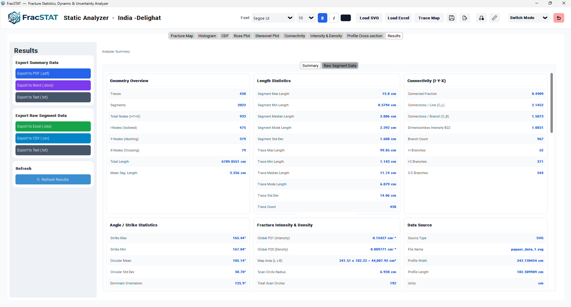
The Results tab occupies the ninth (rightmost) position in the Static Analyzer's main CTkTabview, alongside Fracture Map, Histogram, CDF, Rose Plot, Stereonet Plot, Connectivity, and Intensity & Density. Its layout follows the same two-column convention used throughout the Static Analyzer: a narrow, scrollable left-hand sidebar containing action controls, and a wide right-hand content panel containing the report itself.
2.1 Sidebar (Left Panel)
The sidebar is a vertically scrollable CTkScrollableFrame containing three stacked cards:
| Card | Purpose |
|---|---|
| Export Summary Data | Three buttons that generate a formatted, human-readable report (PDF, Word, or plain text) summarising every statistic computed for the current fracture network. |
| Export Raw Segment Data | Three buttons that export the underlying per-segment table (Excel workbook, CSV, or tab-delimited text) rather than the aggregated statistics. |
| Refresh | A single button that forces an immediate recomputation and redraw of both inner tabs, bypassing the lazy-loading mechanism described in Section 7. |
2.2 Content Panel (Right Panel)
The content panel hosts an inner CTkTabview ("Analyzer Summary") with two pages:
| Page | Contents |
|---|---|
| Summary | A dashboard of thirteen colour-coded statistic cards arranged in a responsive three-column grid, covering geometry, length statistics, connectivity, orientation, intensity/density, data provenance, and the full suite of CDF distribution-fitting results, plus a dynamically rendered Model Comparison table when applicable. |
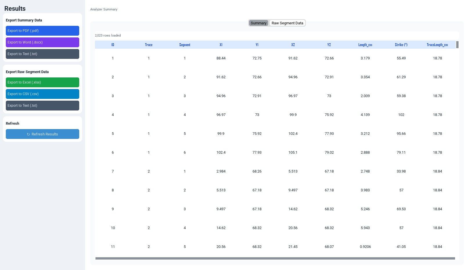
| Raw Segment Data | A sortable, scrollable spreadsheet-style table (a ttk.Treeview widget) listing every computed segment or fracture-plane record with format-appropriate columns. |
3. Data Input and Dependencies
The Results tab has no independent file-loading controls; it consumes state already populated
in the shared StaticAnalyzerApp instance by other tabs after an SVG trace map or
Excel/CSV orientation table has been loaded. The principal upstream data structures it reads
are summarised below.
| Attribute | Populated by | Description |
|---|---|---|
self.results (DataFrame) | run_static_calculations() in static_app.py / static_map_tab.py | One row per computed segment or fracture plane, holding ID, Trace, Segment, X1/Y1/X2/Y2, StrikeDeg, DipDeg, Length_m, Aperture, TraceLengthM, and (for focal-mechanism data) Lat, Lon, EventLabel, PlaneName, Region, BeachballURL. |
self.segments (list[Segment]) | SVG or Excel/CSV loader | Raw parsed segment/plane objects; used to detect whether the source data carries genuine map geometry (_has_map_geometry) for column-set and export-column selection. |
self._fluid_connectivity | Connectivity tab (count_iyx_nodes) | A ConnectivityResult object exposing I/Y/X node arrays, branch counts, and the I-I/I-C/C-C branch classification used for the Connectivity (I-Y-X) statistics block. |
self.p21_stats_labels | Intensity & Density tab | Live CTkLabel widgets already showing the global P21 and P20 values and the scan-circle grid layout; the Results tab reads their displayed text directly rather than recomputing them. |
self.current_stats | CDF tab (_draw_static_cdf) | A flat, ordered dictionary of descriptive and model-fit statistics, including section markers (e.g. "── Power-law ──") used to reconstruct the origin distribution of each entry. |
self._cdf_fit_cache / self._cdf_bootstrap_cache | CDF tab | Internal caches of the most recently computed powerlaw.Fit object and bootstrap confidence-interval/goodness-of-fit results, keyed by a data-and-settings fingerprint; the Results tab reads the most recent entry to backfill every distribution's parameters simultaneously (Section 6.4). |
self.project | Project launcher | Project metadata (name, location, save directory) embedded in exported report headers. |
Because the Results tab is purely a consumer of upstream state, no validation of the source SVG/Excel file occurs here; all format detection, coordinate-system handling, and column validation happens in the SVG/Excel loaders and the Fracture Map tab before any data reaches this module.
4. Settings and Controls
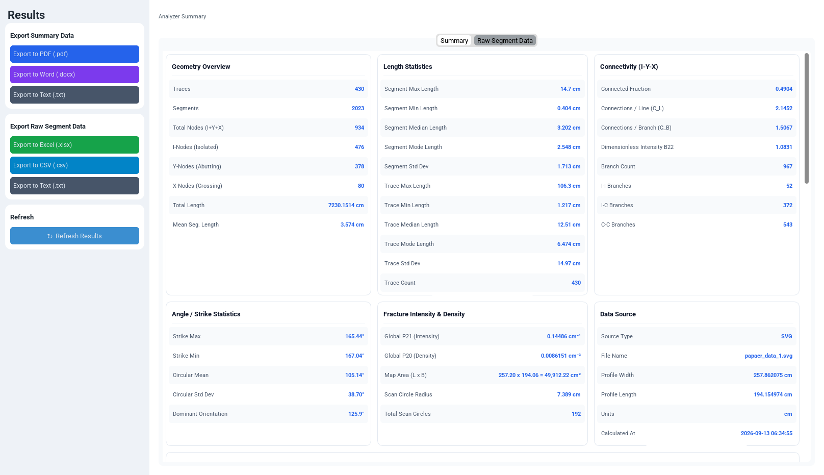
Unlike the plotting tabs, the Results tab exposes no numeric parameters, colour pickers, or sliders — its "settings" are entirely action buttons that trigger export or refresh operations.
4.1 Sidebar Controls
| Control | Card | Action |
|---|---|---|
| Export to PDF (.pdf) | Export Summary Data | Invokes _export_pdf(): renders every statistic section as a two-column ReportLab table inside a formatted A4 document, including the dynamically parsed Model Comparison table when a CDF multi-model comparison has been run. |
| Export to Word (.docx) | Export Summary Data | Invokes _export_word(): builds an equivalent report using python-docx, with native Word heading styles, coloured title text, and Word tables for each statistic section and the comparison table. |
| Export to Text (.txt) | Export Summary Data | Invokes _export_txt(): writes a monospaced, fixed-width plain-text report using the same section ordering, suitable for archiving or diffing between analysis runs. |
| Export to Excel (.xlsx) | Export Raw Segment Data | Invokes _export_excel(): writes the full per-segment/per-plane results DataFrame (after unit-aware column renaming) to a single-sheet .xlsx workbook via openpyxl. |
| Export to CSV (.csv) | Export Raw Segment Data | Invokes _export_csv(): writes the same DataFrame to a comma-separated file using pandas.DataFrame.to_csv. |
| Export to Text (.txt) | Export Raw Segment Data | Invokes _export_raw_txt(): writes the same DataFrame tab-delimited, for import into legacy or non-spreadsheet tools. |
| ↻ Refresh Results | Refresh | Invokes refresh_static_results(force=True), forcing an immediate recompute-and-redraw of both inner tabs even if the tab is not currently visible and no underlying data change has been detected. |
4.2 Inner Tab Controls
The Summary and Raw Segment Data pages are selected via a standard CTkTabview segmented control
at the top of the content panel. No additional filtering, sorting, or display controls are
provided on the Summary page; every statistic card is always shown in full. The Raw Segment
Data page's ttk.Treeview supports native column-header click-to-sort behaviour and
independent horizontal/vertical scrollbars, but exposes no FracSTAT-specific filtering controls.
4.3 Lazy-Loading Behaviour
The Results tab is registered with a wrapped CTkTabview command handler so that the
(potentially expensive) work of populating the dashboard and raw-data table is deferred until
the user actually clicks the Results tab, rather than being recomputed on every geometry change
elsewhere in the workspace. A boolean flag, self._results_stale, is set whenever
refresh_static_results() is called from elsewhere in the application (for example
after loading a new file or changing the profile scale); the flag is only cleared once the tab
is actually visited and _load_results_with_loader() has completed.
5. Mathematical Background
This section defines, with full mathematical notation, every quantity computed or re-derived inside the Results module. Quantities that are computed upstream (in the Histogram, Connectivity, Intensity & Density, or CDF tabs) and simply displayed here are also defined, since the Results tab is where a user most commonly encounters them assembled together for the first time.
5.1 Geometry and Length Statistics
Let the fracture network consist of ns segments grouped into nt traces. For each segment i, let Li denote its length in the project's display unit (m, cm, mm, or km, selected on the Fracture Map tab).
Trace length is the sum of the constituent segment lengths for each trace; per-trace totals are stored in the TraceLengthM column of the results table (or computed on demand as a group-wise sum).
For both the segment-length and trace-length populations, the Results tab reports the maximum, minimum, median, sample standard deviation (using Bessel's correction, ddof = 1), and the statistical mode. Because fracture lengths are continuous, the mode is estimated from a histogram (Section 6.1) rather than from an exact value count.
5.2 Circular (Axial) Orientation Statistics
Fracture strikes are axial data — a fracture measured at azimuth θ is physically indistinguishable from one measured at θ + 180°. Ordinary (linear) circular statistics would therefore be biased; the module instead uses the doubled-angle method for axial data (Mardia and Jupp, 2000, sec. 2.3.4). Each strike θᵢ (already folded into 0°–180°) is doubled to 2θᵢ, mapped onto the full circle, and averaged as a set of unit vectors:
R (the mean resultant length, 0 ≤ R ≤ 1) measures the concentration of the strike population: R close to 1 indicates a strongly preferred orientation (a single dominant fracture set), while R close to 0 indicates near-uniform, poorly organised orientations. The Dominant Orientation statistic reported alongside the circular mean is instead the histogram-modal bin centre (Section 6.1) — it can differ from the circular mean whenever the strike distribution is multi-modal (e.g. two conjugate fracture sets), since the circular mean of two symmetric peaks straddling a gap is not itself a peak.
5.3 Connectivity and Topology (I-Y-X Node Theory)
The connectivity statistics implement the standard structural-geology I-Y-X node classification (Sanderson and Nixon, 2015); the node and branch terminology follows the fracture-network glossary (Peacock et al., 2016). Classification is performed at trace level, not segment level: a trace's only tips are the start of its first segment and the end of its last, and the interior vertices of a digitised polyline are not nodes at all. Each node is then one of three types, distinguished by how many branches meet there:
| Node Type | Symbol | Branches | Geological Meaning |
|---|---|---|---|
| Isolated | I | 1 | A free-standing fracture tip that terminates without abutting or crossing another fracture; contributes nothing to fluid connectivity at that point. |
| Abutting | Y | 3 | One fracture tip terminates against the interior of another (a T- or Y-shaped junction); a single-sided hydraulic connection. |
| Crossing | X | 4 | Two fracture interiors cross one another, each continuing beyond the intersection; a fully connected, four-way hydraulic junction. |
Two tips that merely touch are not a node. Only two branches meet at such a contact, so it is none of I, Y, or X; both tips remain I nodes and the contact itself is not counted. Recording it as a Y would add three branch-ends where only two exist and break the node-degree identity below, leaving a non-integer N_B.
Let N_I, N_Y, N_X denote the counts of each node type. Two derived connectivity indices are computed:
C_L and C_B are the average-connections-per-line and average-connections-per-branch indices of Sanderson and Nixon (2015, eqs. 4–8); both increase toward their theoretical maxima (4 for C_L on a fully crossing network, 2 for C_B) as the network becomes progressively better connected. The N_B expression is the node-degree identity: each I node terminates one branch, each Y node three, each X node four, and every branch has exactly two ends, hence the division by two. It follows that N_B is always an integer for a correct classification — a fractional value is a diagnostic that some contact has been given the wrong node type.
The Connected Fraction reported in the summary is (N_Y + N_X) / (N_I + N_Y + N_X), i.e. the proportion of nodes that are not simply dead-end tips.
Branch Count and C_B come from different computations, on purpose. The
Branch Count, I-I, I-C, and C-C fields are
ConnectivityResult.branch_count and its census, obtained by walking each trace
and cutting it at its nodes. C_B, by contrast, divides by the N_B implied by the node
identity above. On a fully sampled network the two agree; they diverge when boundary I nodes
have been censored on the Connectivity tab, because the node formula has no way to add back
the removed tips. Reading the two side by side is therefore the genuine internal
cross-check, and a mismatch here means boundary censoring is active rather than that
something is wrong.
A branch is the portion of a trace lying between two adjacent nodes (of any type) — it is a topological object, so an isolated trace drawn with one segment and the same trace drawn with fifty both contain exactly one branch. Every branch is classified by the type of node at each of its two ends into one of three topological classes: I-I (isolated at both ends), I-C (isolated at one end, connected — Y or X — at the other), and C-C (connected at both ends). Their counts, nII, nIC, nCC, are reported directly, sum to the Branch Count, and feed the branch-topology (Sanderson) ternary diagram on the Connectivity tab. The Dimensionless Intensity, B22, is the branch-normalised intensity of Sanderson and Nixon (2015, eq. 9):
read from ConnectivityResult.dimensionless_branch_intensity. Because the
denominator carries the topological branch count, B22 is invariant to digitisation density; a
raw segment count in its place would make the value fall as the same traces were drawn with
more vertices. Note that the Sample Area here is the Connectivity tab's sampling window when
one has been entered, which need not equal the Map Area (L x B) field reported in the
Fracture Intensity & Density card — that field is always the data's own bounding box.
5.4 Fracture Intensity and Density (P21, P20)
The Results tab does not recompute these: it reads the text of the Intensity & Density tab's Global Intensity (P21) and Global Density (P20) labels verbatim, so the values are the network-wide definitions applied to the mapped bounding box, not per-circle estimates:
P20 counts whole traces (df["Trace"].nunique()), following the
Pij definition of Dershowitz and Herda (1992) in which the density of
zero-dimensional features is a count of fractures per unit area. A digitised-segment count in
its place would report a density proportional to how finely the traces were drawn — ten times
too high for traces stored as ten segments each — while leaving P21 unaffected, since summed
length telescopes over polyline vertices.
The spatially resolved grids on the Intensity & Density tab do use the Mauldon circular-window estimators, I = N/(4r) from boundary crossings and D = M/(2πr²) from trace tips inside the circle (Mauldon et al., 2001); those are unbiased with respect to fracture orientation, because a circular sampling window intersects fractures of every strike with equal probability (cf. Terzaghi, 1965). The Results tab reports the Scan Circle Radius r and Total Scan Circles that produced them, but reproduces only the two global scalars above.
5.5 Probability Distribution Fitting (CDF Backfill)
The Results tab reproduces the parameters, information criteria, and goodness-of-fit statistics of every maximum-likelihood distribution model fitted on the CDF tab: Power-law, Exponential, Log-normal, Weibull (implemented as a stretched exponential), and Truncated Power-law. The complete mathematical derivation of these fits (log-likelihood construction, AIC/AICc/BIC, Kolmogorov–Smirnov statistics, bootstrap confidence intervals, and the parametric bootstrap goodness-of-fit p-value) follows the maximum-likelihood framework of Clauset, Shalizi and Newman (2009) and is the responsibility of the CDF tab, where it is documented; the Results tab's role is purely to surface the cached fit object's parameters into the dashboard. For completeness, the defining forms of each survival function P(L>x) for x ≥ x_min are:
6. Algorithms
6.1 Histogram-Based Mode Estimation
Because fracture segment/trace lengths and strike angles are continuous quantities, the module
estimates the statistical mode by binning the data with numpy.histogram using the
same bin count as the Histogram tab's own control (falling back to 20 bins if that control has
not yet been built), then returning the centre of whichever bin holds the highest count. If the
data range degenerates to a single value (max equals min), that value is returned directly.
This histogram-derived mode is reused for three quantities: Segment Mode Length, Trace Mode
Length, and the Dominant Orientation (Strike) bin centre.
def _histogram_mode(values_arr: np.ndarray, n_bins: int) -> float:
    if values_arr.size == 0:
        return 0.0
    v_min, v_max = float(values_arr.min()), float(values_arr.max())
    if v_min == v_max:
        return v_min
    step = (v_max - v_min) / n_bins
    centres = np.arange(v_min, v_max + step / 2, step)
    edges = np.concatenate([[centres[0] - step / 2], centres + step / 2])
    counts, _ = np.histogram(values_arr, bins=edges)
    if counts.size == 0:
        return v_min
    return float(centres[int(np.argmax(counts))])
The _histogram_mode() helper, shared by the Segment Mode Length, Trace Mode Length, and Dominant Orientation statistics.
6.2 Dynamic Column-Set Resolution for Raw Data Export
Because FracSTAT accepts several structurally different input formats (SVG trace geometry,
spatial Excel/CSV tables, legacy orientation-only fracture-plane tables, and Global CMT-style
focal-mechanism tables), the Results tab cannot assume a fixed set of columns exists in
self.results. The _raw_data_column_set() algorithm inspects the
loaded segment objects to determine which of three column templates applies:
| Detected Format | Detection Rule | Displayed / Exported Columns |
|---|---|---|
| Focal mechanism | Lat column present and at least one non-null value | ID, Trace, PlaneName, EventLabel, Region, Lat, Lon, StrikeDeg, DipDeg, Rake |
| Orientation-only | segments[0]._has_map_geometry is False | ID, Trace, Segment, StrikeDeg, DipDeg, Length_m, Aperture |
| Spatial (SVG or coordinate-bearing Excel) | default / has_geometry True | ID, Trace, Segment, X1, Y1, X2, Y2, Length_m, Aperture, StrikeDeg, TraceLengthM |
def _raw_data_column_set(self, df):
    segs = getattr(self, "segments", None)
    has_geometry = getattr(segs[0], "_has_map_geometry", True) if segs else True
    has_latlon = "Lat" in df.columns and df["Lat"].notna().any()

    if has_latlon:
        candidates = ["ID", "Trace", "PlaneName", "EventLabel", "Region",
                      "Lat", "Lon", "StrikeDeg", "DipDeg", "Rake"]
    elif not has_geometry:
        candidates = ["ID", "Trace", "Segment", "StrikeDeg", "DipDeg",
                      "Length_m", "Aperture"]
    else:
        candidates = ["ID", "Trace", "Segment", "X1", "Y1", "X2", "Y2",
                      "Length_m", "Aperture", "StrikeDeg", "TraceLengthM"]

    display_cols = [c for c in candidates if c in df.columns]
    if not display_cols:
        display_cols = [c for c in df.columns if c != "Color"]
    return display_cols
Only columns that are actually present in the DataFrame are retained; if none of the candidate
columns exist (an unexpected edge case) the routine falls back to displaying every column
except the internal Color field. The same three-way branching, together with a DipDeg-drop rule
(removing the DipDeg column entirely when every value is the default 90° placeholder) and a
geometry-column drop for orientation-only data, is applied a second time inside
_get_export_df() before Excel/CSV/Text export, so the exported spreadsheet never
contains meaningless placeholder geometry.
6.3 Unit-Aware Column Renaming
Before both on-screen display and file export, length-bearing columns are renamed to embed the
currently selected display unit, e.g. Length_m becomes Length_cm when
the user has selected centimetres on the Fracture Map tab's unit selector, and
TraceLengthM becomes TraceLength_km for kilometres. This prevents
ambiguity when a user changes units mid-session or shares an exported file with a collaborator.
6.4 CDF Model Backfill from the Fit Cache
Rather than re-running the (potentially slow) maximum-likelihood fitting procedure,
_collect_cdf_summary_values() reads the most recently computed entry from the CDF
tab's internal fit cache (self._cdf_fit_cache) — a dictionary keyed by a
fingerprint of the input data and the active fitting settings — and extracts the
powerlaw.Fit object's five sub-model attributes (power_law,
exponential, lognormal, stretched_exponential,
truncated_power_law) directly. From that single cached fit, the algorithm
reconstructs, for every one of the five distributions simultaneously, its fitted parameter(s),
95% (or user-selected level) bootstrap confidence interval (if a bootstrap run has been
performed), tail sample size and percentage, log-likelihood, AIC, BIC, the powerlaw library's
native Kolmogorov–Smirnov D statistic, an independently computed SciPy asymptotic KS statistic
and p-value, and — if available — the parametric-bootstrap goodness-of-fit p-value. This
backfill approach means the Results tab always shows every candidate distribution's statistics
side by side, even though the CDF tab's own plot only ever actively displays the single model
currently selected in its dropdown.
6.5 Textual current_stats Parsing
A second pass over the CDF tab's self.current_stats dictionary (an ordered, flat
dictionary populated live as the CDF tab redraws) recovers information that is not part of the
cached Fit object itself: the raw descriptive statistics block, any manually overridden
Truncated Power-law parameters (α, λ fixed by the user rather than found by MLE), bootstrap
confidence-interval strings, and — when present — the full Model Comparison / Auto Best Fit
narrative text and pairwise likelihood-ratio table. Section markers in the dictionary (keys
formatted as "── SectionName ──") are used to prefix subsequent keys with their originating
distribution name (e.g. turning a bare "xmin" key into "Power-law xmin"), except for the
Descriptive, Auto Best Fit, and Model Comparison sections, whose keys are already
self-describing and are left unprefixed.
6.6 Dynamic Comparison-Table Rendering
When a CDF Model Comparison or Auto Best Fit run has been performed, its result is a
pipe-delimited (|) plain-text table embedded as a single multi-line string value under the key
"Comparison Table". The Results tab's _render_comparison_table() parses this
string line by line: lines containing at least one pipe character are split into cells and
rendered as a horizontally scrollable grid (alternating row shading, bold header row); lines
without a pipe character (dashed separators are skipped, footnote/interpretation lines are
kept) are rendered as italicised note paragraphs beneath the grid. The identical parsing logic
is duplicated, with format-appropriate output primitives, inside the PDF export (ReportLab
Table/Paragraph objects) and the Word export (python-docx table rows) so that the printed
report matches the on-screen dashboard exactly.
7. Internal Workflow
The Results tab participates in the application-wide tab-change and dirty-tracking machinery
already used by the other Static Analyzer tabs, extended with its own staleness flag so that
its two moderately expensive population routines — _populate_summary() and
_populate_raw_data() — are only ever run when actually needed.
7.1 Construction Sequence
_build_static_results_tab()is called once, during workspace start-up, after every other tab has been built. It constructs the sidebar cards, the inner Summary/Raw Segment Data tabview, and every statistic-card label placeholder (each pre-populated with the em-dash "—" as a not-yet-computed sentinel).- It then wraps the outer CTkTabview's existing on-tab-change command (which already performs
autosave and other bookkeeping for the other tabs) with an additional check: if the newly
selected tab is "Results" and
self._results_staleis True,_load_results_with_loader()is invoked. self._results_staleis initialised to True, so the very first visit to the Results tab always performs a full population, regardless of whether any data has been loaded yet (in which case the population routines simply render their respective empty states).
self._results_stale = True

existing_cmd = self.tabs.cget("command")
def _on_tab_click():
    if existing_cmd:
        existing_cmd()
    if self.tabs.get() == "Results" and getattr(self, "_results_stale", False):
        self._load_results_with_loader()

self.tabs.configure(command=_on_tab_click)
The wrapped tab-change command installed at the end of _build_static_results_tab(), chaining onto whatever command the CTkTabview already had.
7.2 Staleness Propagation
refresh_static_results(force=False) is the single external entry point other
parts of the workspace call whenever underlying data changes (e.g. at the end of the
multi-step refresh_all_tabs() chain in static_app.py, itself
triggered after loading a new SVG/Excel file, changing the profile scale, or editing the
Y-axis azimuth). It always sets self._results_stale = True. If
force=True (used by the explicit Refresh button) or the Results tab already
happens to be the active tab, it immediately calls _load_results_with_loader();
otherwise it only updates a small status label ("Data changed. Click tab to load.") and clears
the raw-data table, deferring the actual work until the user next clicks the tab.
7.3 Loader Routine
_load_results_with_loader() shows the shared global loading overlay ("Compiling
Results Data…"), then — after a short after() delay so the overlay has a chance
to paint before the main thread is blocked — calls _populate_summary() followed
by _populate_raw_data(), clears the stale flag, and hides the overlay. Both
population routines run synchronously on the Qt main thread; no background threading is
used for the Results tab itself (unlike the SVG/Excel loaders in the Fracture Map tab, which do
use worker threads for the geometry recomputation that feeds this tab).
7.4 Summary Population
_populate_summary() calls _collect_all_summary_values() to build a
single flat dictionary of every statistic (merging the geometry/connectivity/intensity
computations described in Section 6 with the CDF backfill dictionary from
_collect_cdf_summary_values()), then walks every pre-built label reference in
self._summary_section_refs, looking up and writing the corresponding formatted
string (or the em-dash placeholder if the key is absent for the current dataset). Finally, it
clears and, if applicable, rebuilds the dynamic Model Comparison table beneath the main grid of
cards.
7.5 Raw Data Population
_populate_raw_data() first tears down any previously built ttk.Treeview
(since the column set can legitimately change between loads — e.g. switching from an SVG file
to a focal-mechanism Excel table), determines the appropriate column set via
_raw_data_column_set() (Section 6.2), configures ttk.Style Treeview colours to
track the current qtk light/dark appearance, and inserts one row per DataFrame record
with values pre-formatted by _raw_fmt_value() (four-significant-figure formatting
for floats, an em-dash for missing values, and unmodified strings otherwise).
def _raw_fmt_value(val):
    if isinstance(val, float):
        if pd.isna(val):
            return "—"
        return f"{val:.4g}"
    if val is None or (isinstance(val, str) and not val.strip()):
        return "—"
    return str(val)
The value-formatting helper used for every cell inserted into the Raw Segment Data Treeview.
8. Statistical Methods
The Results tab presents statistics from four broad families: descriptive geometry statistics, circular orientation statistics, discrete topological (graph-theoretic) connectivity statistics, and parametric probability-distribution fitting statistics for the tail of the fracture-length distribution. The table below inventories every statistical quantity shown on the Summary dashboard, its source, and its interpretation.
| Card | Field | Statistical Meaning |
|---|---|---|
| Geometry Overview | Traces / Segments / Total Nodes | Sample sizes: number of distinct fracture traces, constituent straight segments, and I+Y+X topological nodes. |
| Length Statistics | Max / Min / Median / Mode / Std Dev | Univariate descriptive statistics of the segment-length and trace-length distributions (Section 5.1). |
| Angle / Strike Statistics | Circular Mean / Circular Std Dev / Dominant Orientation | Axial circular statistics of the doubled-angle strike distribution (Section 5.2). |
| Connectivity (I-Y-X) | Connected Fraction / C_L / C_B / B22 / Branch Count / Branch classes | Topological connectivity indices from trace-level I-Y-X node theory; Branch Count is the trace-walk census, C_B the node-derived one (Section 5.3). |
| Fracture Intensity & Density | Global P21 / Global P20 / Map Area / Scan Circle Radius | Network-wide length-per-area and traces-per-area over the mapped bounding box, mirrored from the Intensity & Density tab, plus the scan-circle geometry behind its Mauldon grids (Section 5.4). |
| CDF: Descriptive Statistics | n, Min, Q1, Median, Q3, Max, IQR, Mean, Std Dev, Variance, CV, Skewness, Kurtosis | Standard order statistics and unbiased higher-moment shape statistics of the fracture-length sample. |
| CDF: Power-law / Exponential / Log-normal / Weibull / Truncated Power-law | α, λ, μ, σ, β, xmin, n_tail, Log-likelihood, AIC, BIC, KS statistic, KS p-value, bootstrap CI, GOF p-value | Maximum-likelihood fit parameters and model-adequacy diagnostics for each of the five candidate tail distributions (Section 5.5). |
| CDF: Model Comparison / Best Fit | Final Recommendation, Recommended Models, Model-Averaging Support, Selection Basis, Selection Warning | Outcome of the CDF tab's multi-criterion model-selection procedure (agreement of AIC/AICc, BIC, KS rank, and pairwise likelihood-ratio tests) as computed and cached by the CDF tab. |
All AIC values use the small-sample-corrected AICc form when the ratio of tail sample size to number of free parameters falls below 40, matching the recommendation of Burnham and Anderson (2002) for model selection with limited data; AIC and BIC themselves are the criteria of Akaike (1974) and Schwarz (1978), and the pairwise likelihood-ratio comparison is the non-nested test of Vuong (1989). This correction and the underlying rationale are implemented and documented in the CDF tab, and simply reported verbatim here.
9. Visualization
9.1 Summary Dashboard Layout
The Summary page uses a three-column, uniform-width CTkScrollableFrame grid. Each statistic family is rendered as an independently bordered, rounded-corner "card" containing a bold section header, a thin divider rule, and a two-column key/value grid with alternating subtle row shading for readability. Card placement follows a fixed (row, column, column-span) layout: the Geometry Overview, Length Statistics, and Connectivity cards occupy the first row (one card per column); Angle/Strike Statistics, Fracture Intensity & Density, and Data Source occupy the second row; the CDF Descriptive Statistics card spans the full three-column width in the third row (reflecting its larger field count); and the five per-distribution CDF cards plus the Model Comparison/Best Fit card occupy the fourth and fifth rows.
Every key/value row is bound to a <Configure> event that recomputes
wraplength for both the field-name and value labels proportionally to the row's live pixel
width, so that long field names (e.g. "Truncated Power-law GOF p-value (bootstrap, refit KS)")
remain fully readable at any window size without being clipped or overlapping the adjacent
value column.
9.2 Comparison Table Widget
When rendered, the dynamic Model Comparison table (Section 6.6) appears beneath the main card grid inside its own bordered card, using a horizontally scrollable CTkScrollableFrame so that wide multi-column comparison tables (Distribution, k, Log-Likelihood, KS, KS p, AIC, ΔAIC, AICc, BIC, ΔBIC, Akaike weight, BIC weight, LRT R, LRT p, Rank, Recommendation — sixteen columns) remain fully navigable without shrinking individual cell text below legibility.
9.3 Raw Segment Data Table
The Raw Segment Data page renders a native ttk.Treeview configured with a
65-pixel row height (tall enough to display two-line wrapped text where needed), synchronized
vertical and horizontal ttk.Scrollbar widgets, and Treeview/Treeview.Heading
ttk.Style rules that adapt background, foreground, and selection-highlight colours to the
current qtk appearance mode. Column widths are set individually per field (130 px for
text-heavy fields such as EventLabel, PlaneName, and Region; 90 px for numeric fields), and
column headings display the unit-qualified name for length fields.
10. Advanced Features
10.1 Multi-Format Report Generation
The three summary-export routines (_export_pdf, _export_word,
_export_txt) all draw from the identical section/field ordering list, guaranteeing
that a PDF, Word, and plain-text export of the same analysis session are structurally identical
in content and section order, differing only in their native formatting idioms (ReportLab
flowables and TableStyle for PDF; python-docx Heading/Table objects with RGBColor-styled runs
for Word; fixed-width padded strings for text). This consistency is a deliberate design choice
so that a laboratory or consultancy can standardise on any one of the three formats without
losing information relative to the others.
10.2 Condensed Comparison-Table Typography for PDF
Because the Model Comparison table can carry up to sixteen columns, the PDF exporter uses a markedly smaller (5.5 pt) Paragraph-wrapped font for its cells (versus the 9–10 pt body font used elsewhere in the same document) and lets ReportLab auto-size column widths, so that the full comparison table fits within an A4 page without truncation. The Word exporter applies an equivalent reduction (6.5 pt) together with centre-aligned cell paragraphs for the same reason.
10.3 Unicode Superscript Normalisation
Several statistics (notably the P21/P20 intensity and density units, e.g. "m⁻¹" and "m⁻²") are rendered with true Unicode superscript characters for on-screen display, since Qt labels support arbitrary Unicode glyphs. Both the PDF and text/Word exporters proactively replace these Unicode superscripts with ASCII-safe equivalents ("^-1", "^-2", "^2") before writing them into the exported document, avoiding missing-glyph rendering issues in some PDF viewers or older Word installations.
# Clean unicode superscripts for safe Word rendering
raw_val = str(summary.get(f, "—"))
clean_val = raw_val.replace("⁻¹", "^-1").replace("⁻²", "^-2").replace("²", "^2")
row_cells[1].text = clean_val
Excerpt from _export_word() showing the superscript-normalisation step applied to every value cell.
10.4 Fingerprint-Based Change Detection
To avoid unnecessary recomputation, several upstream tabs (most notably the CDF tab, whose MLE fitting is the single most expensive computation in the whole workspace) use a lightweight fingerprint — typically (row count, rounded sum of a key numeric column, active setting values) — to decide whether a data-dependent cache entry is still valid. The Results tab's backfill logic in Section 6.4 relies on, and benefits from, this same caching discipline: it never triggers a new distribution fit itself, so opening the Results tab is always fast, but it always reflects whatever the most recent CDF computation produced.
11. Performance Optimization
| Technique | Where Applied | Effect |
|---|---|---|
| Lazy tab population | Whole module (Section 7) | Avoids running _populate_summary()/_populate_raw_data() on every keystroke or data change elsewhere in the workspace; work happens only when the user actually views the Results tab. |
Global loading overlay with deferred after() call | _load_results_with_loader() | Gives the Qt event loop one paint cycle to render the overlay before the (synchronous) population routines run, so the UI never appears to freeze without feedback. |
| Reuse of the CDF tab's fit and bootstrap caches | _collect_cdf_summary_values() | Backfills five complete distribution-fit summaries without invoking powerlaw.Fit a second time; the expensive MLE optimisation (and, if enabled, the n-bootstrap-resample CI/GOF loop) is computed exactly once regardless of how many times the Results tab is refreshed. |
| Treeview full teardown/rebuild only on population | _populate_raw_data() | The Treeview is destroyed and recreated only when the tab is actually repopulated (not on every resize or scroll), keeping the raw-data view responsive for networks with hundreds to low thousands of segments. |
| Row-capped display convention elsewhere in the app is not applied here | Raw Segment Data table | Unlike the Dynamic Analyzer's Table tab (which caps rows at 1000 for interactivity), the Results tab's raw-data export and display are intended as a complete scientific record and are not truncated; very large networks may therefore take longer to populate this tab than the interactive plotting tabs. |
12. Practical Examples
12.1 Example 1 — Verifying a Newly Loaded SVG Trace Map
- Load an SVG fracture trace map via the Fracture Map tab's Load SVG button, and confirm the map renders as expected.
- Open the Connectivity tab once to trigger its (independently lazy) I-Y-X computation, since the Results tab's Connectivity card depends on that cache being populated.
- Click the Results tab. Confirm the Geometry Overview card's Traces count matches the number of distinct traces visible on the map (Segments will be larger whenever traces were digitised as polylines), and sanity-check the node census against twice the trace count: every trace has exactly two tips, so N_I cannot exceed 2 × Traces, and each Y or X consumes tips or interiors from that budget. Then check that (N_I + 3N_Y + 4N_X) / 2 is a whole number — a fractional result means a contact has been mis-typed.
- Inspect the Length Statistics card: an unexpectedly large Segment Max Length relative to the Median often indicates a digitising error (e.g. two traces that should have been separate objects were accidentally merged into one long path during SVG creation).
- Export the summary as a PDF for inclusion in a field-mapping QC report using Export to PDF (.pdf).
12.2 Example 2 — Selecting a Length Distribution Model for Reporting
- On the CDF tab, set Distribution Fit Model to Auto Best Fit and, optionally, enable Bootstrap CI & GOF with a chosen resample count.
- Switch to the Results tab. The CDF: Power-law, CDF: Exponential, CDF: Log-normal, CDF: Weibull, and CDF: Truncated Power-law cards will all be populated simultaneously from the single cached fit, letting every candidate model's AIC, BIC, and KS statistic be compared at a glance without switching the CDF tab's dropdown five times.
- Read the CDF: Model Comparison / Best Fit card's Final Recommendation and Selection Warning fields to determine whether the automatic procedure found a statistically unambiguous winner or whether several models remain practically indistinguishable (in which case the recommended approach is to report the model-averaged parameter estimates shown under Model-Averaging Support rather than a single "best" model).
- Scroll to the dynamically rendered Comparison Table beneath the card grid for the full pairwise likelihood-ratio evidence underlying that recommendation, then export the whole page to Word for inclusion in a manuscript's supplementary materials.
12.3 Example 3 — Exporting Raw Data for External GIS or Statistical Software
- Switch to the Raw Segment Data inner tab and confirm the displayed column set matches the loaded data format (spatial X1/Y1/X2/Y2 columns for SVG data; Lat/Lon/PlaneName for a focal-mechanism table).
- Use Export to CSV (.csv) in the sidebar to produce a file directly importable into GIS software (e.g. QGIS) for spatial cross-referencing against other datasets, or Export to Excel (.xlsx) for further manual analysis in a spreadsheet.
13. Geological Interpretation
The Results dashboard is designed to answer, in one screen, the questions a structural geologist or reservoir engineer typically asks of a digitised fracture network.
13.1 Is the network well connected?
High values of Connected Fraction and C_L/C_B, together with a large proportion of X and C-C nodes relative to I nodes, indicate a network capable of supporting significant fluid or gas through-flow — relevant to reservoir permeability, contaminant transport, and slope-stability seepage analysis. A network dominated by I nodes and I-I branches, by contrast, behaves closer to a set of isolated, disconnected discontinuities.
13.2 Is the network scale-invariant (fractal) or does it have a characteristic length?
A Power-law fit with a low AIC/BIC relative to the Exponential and Log-normal alternatives, combined with a high KS p-value, supports treating the fracture-length population as approximately scale-invariant over the sampled range — a common finding for tectonic joint sets (Bonnet et al., 2001) and consistent with self-similar brittle deformation processes; note that the scaling range is itself usually finite (Marrett et al., 1999). An Exponential or Log-normal preference instead suggests a characteristic length scale exists, often associated with mechanical layer thickness control on fracture propagation (bed-confined jointing) or a specific genetic mechanism with a finite driving-stress range.
13.3 Does the network show a preferred orientation, and how strong is it?
A low Circular Std. Dev. paired with a Dominant Orientation close to the Circular Mean indicates a single, tectonically controlled fracture set (e.g. joints formed under a consistent regional stress field). A high circular standard deviation, or a Dominant Orientation that diverges substantially from the circular mean, is a signature of either two conjugate sets or a poorly organised, possibly non-tectonic (e.g. cooling-joint or weathering-related) fracture population — best confirmed by cross-checking against the Rose Plot tab.
13.4 How intense is fracturing, and is it representative of the true rock mass?
P21 and P20 provide areal-density measures directly comparable across different outcrops, scanlines, or digital elevation models, because the Mauldon circular-scanline method removes the orientation bias inherent in straight-line scanline sampling (the classical Terzaghi correction problem) (Terzaghi, 1965; Mauldon et al., 2001). Comparing P21 values between multiple mapped domains within the same project is a standard way to identify structural domains or damage zones associated with faults, though the comparison is only as representative as the sampling scheme behind it (Watkins et al., 2015).
14. Implementation Notes
- The module is implemented as a Python mixin class (
StaticResultsTab) intended to be combined via multiple inheritance withStaticAnalyzerAppand its sibling tab mixins; it therefore freely reads and writes attributes (self.results,self.segments,self._fluid_connectivity,self.current_stats, and others) that are defined by those sibling classes rather than by itself. - All numeric formatting in the Summary dashboard uses Python's general (
%.4g) or fixed-precision (%.4f,%.3f) format specifiers chosen per-field to balance readability against precision; users requiring full machine precision should use the raw-data or CDF-tab-native exports rather than the formatted Summary text. - PDF export depends on the
reportlabpackage; Word export depends onpython-docx; both are optional dependencies and their absence is caught and reported to the user via a friendly "Missing library" message box rather than a raw stack trace. - Excel export depends on
openpyxl, again with a graceful ImportError message. - The export file-save dialog defaults its initial directory to the application-wide configured export path (Settings page → Export → Default export directory) when one has been configured and still exists on disk, falling back to the operating system's default save location otherwise.
- Because the CDF backfill (
_collect_cdf_summary_values) reads only the most recently cached fit-cache entry, switching the CDF tab's data source (e.g. from Segment Lengths to Trace Total Lengths) or its fitting cutoff (x_min mode) and then immediately visiting the Results tab without letting the CDF tab redraw first can momentarily show statistics computed under the previous settings; visiting the CDF tab at least once after any such change ensures the cache — and therefore the Results tab — reflects the new settings.
15. Limitations
| Limitation | Description |
|---|---|
| No independent CDF computation | The Results tab performs no independent statistical computation for the CDF distribution-fitting section; it is entirely dependent on the CDF tab having been visited (so that its fit cache is populated) at least once during the current session. If no CDF fit has ever been run, the five per-distribution cards remain blank (em-dash placeholders). |
| Mode estimates are bin-count sensitive | Histogram-derived mode estimates (Section 6.1) are sensitive to the chosen bin count; because that bin count is shared with the Histogram tab's own control, changing it there will change the reported Mode values here on the next refresh, which is expected behaviour but can surprise users unaware of the shared setting. |
| Two areas are reported, and they need not agree | Map Area (L x B) is always the data's own bounding box, recomputed here from the X1/X2/Y1/Y2 extremes. B22, however, normalises by ConnectivityResult.sample_area, which is the sampling window entered on the Connectivity tab whenever one has been supplied. If a window smaller or larger than the trace extent is in use, the two figures differ by design; the B22 value is the one tied to the window, and P21/P20 are the ones tied to the bounding box. |
| Connectivity fields depend on the Connectivity tab having run | All I-Y-X, branch, and B22 fields read self._fluid_connectivity; if count_iyx_nodes() has not been run in the current session they fall back to zeros rather than blanks, so a genuine all-zero connectivity block and a not-yet-computed one look the same. Boundary I-node exclusion and the snap tolerance in force on that tab also propagate here silently. |
16. References
Sources are listed alphabetically within each group. In-text citations throughout this page link to the corresponding entry below.
16.1 Fracture Intensity, Topology and Sampling
- Dershowitz, W. S., & Herda, H. H. (1992). Interpretation of fracture spacing and intensity. In Proceedings of the 33rd U.S. Symposium on Rock Mechanics (pp. 757–766). Balkema, Rotterdam. ISBN 978-90-5410-045-3. (Source of the Pij notation; P20 is a count of fractures per unit area.)
- Mauldon, M., Dunne, W. M., & Rohrbaugh, M. B. (2001). Circular scanlines and circular windows: new tools for characterizing the geometry of fracture traces. Journal of Structural Geology, 23(2–3), 247–258. https://doi.org/10.1016/S0191-8141(00)00094-8
- Peacock, D. C. P., Nixon, C. W., Rotevatn, A., Sanderson, D. J., & Zuluaga, L. F. (2016). Glossary of fault and other fracture networks. Journal of Structural Geology, 92, 12–29. https://doi.org/10.1016/j.jsg.2016.09.008
- Sanderson, D. J., & Nixon, C. W. (2015). The use of topology in fracture network characterization. Journal of Structural Geology, 72, 55–66. https://doi.org/10.1016/j.jsg.2015.01.005 (I-Y-X nodes; C_L, C_B and B22.)
- Terzaghi, R. D. (1965). Sources of error in joint surveys. Géotechnique, 15(3), 287–304. https://doi.org/10.1680/geot.1965.15.3.287
- Watkins, H., Bond, C. E., Healy, D., & Butler, R. W. H. (2015). Appraisal of fracture sampling methods and a new workflow to characterise heterogeneous fracture networks at outcrop. Journal of Structural Geology, 72, 67–82. https://doi.org/10.1016/j.jsg.2015.02.001
16.2 Distribution Fitting and Model Selection
- Akaike, H. (1974). A new look at the statistical model identification. IEEE Transactions on Automatic Control, 19(6), 716–723. https://doi.org/10.1109/TAC.1974.1100705
- Burnham, K. P., & Anderson, D. R. (2002). Model Selection and Multimodel Inference: A Practical Information-Theoretic Approach (2nd ed.). Springer, New York. https://doi.org/10.1007/b97636 (AICc when n/K < 40; Akaike weights.)
- Clauset, A., Shalizi, C. R., & Newman, M. E. J. (2009). Power-law distributions in empirical data. SIAM Review, 51(4), 661–703. https://doi.org/10.1137/070710111
- Schwarz, G. (1978). Estimating the dimension of a model. The Annals of Statistics, 6(2), 461–464. https://doi.org/10.1214/aos/1176344136
- Vuong, Q. H. (1989). Likelihood ratio tests for model selection and non-nested hypotheses. Econometrica, 57(2), 307–333. https://doi.org/10.2307/1912557
16.3 Fracture-Length Scaling and Directional Statistics
- Bonnet, E., Bour, O., Odling, N. E., Davy, P., Main, I., Cowie, P., & Berkowitz, B. (2001). Scaling of fracture systems in geological media. Reviews of Geophysics, 39(3), 347–383. https://doi.org/10.1029/1999RG000074
- Mardia, K. V., & Jupp, P. E. (2000). Directional Statistics. John Wiley & Sons. https://doi.org/10.1002/9780470316979 (Sec. 2.3.4: doubled-angle summaries for axial data.)
- Marrett, R., Ortega, O. J., & Kelsey, C. M. (1999). Extent of power-law scaling for natural fractures in rock. Geology, 27(9), 799–802. https://doi.org/10.1130/0091-7613(1999)027<0799:EOPLSF>2.3.CO;2
Methods statement for the Results tab. The Results tab performs no independent fitting; it surfaces values computed elsewhere in the Static Analyzer. If a table exported from it appears in a publication, the details below are what a reader needs, and are what the citations above assume:
Strike summaries are axial circular statistics computed on doubled angles (Mardia and Jupp, 2000). Connectivity indices are the trace-level I-Y-X node counts and the derived C_L, C_B and B22 of Sanderson and Nixon (2015), with node and branch terms as defined by Peacock et al. (2016). Global intensity and density use the Pij convention (Dershowitz and Herda, 1992) over the data bounding box, with P20 counting whole traces; the orientation-unbiased circular-window estimators are reported on the Intensity & Density tab (Mauldon et al., 2001; cf. Terzaghi, 1965). Length-distribution parameters are maximum-likelihood tail fits with xmin selection and bootstrap goodness of fit (Clauset et al., 2009), ranked by AIC/AICc (Akaike, 1974; Burnham and Anderson, 2002), BIC (Schwarz, 1978) and non-nested likelihood-ratio tests (Vuong, 1989). Report the sampling window used for B22 separately from the bounding box used for P21/P20, since the two need not agree, and state that scale-invariance claims apply only over the fitted range (Marrett et al., 1999; Bonnet et al., 2001). Because reported values depend on whether the CDF and Connectivity tabs have been run, and on the sampling scheme itself (Watkins et al., 2015), record the session settings alongside any exported summary.