Dynamic Rose Tab
Located at dynamic_analyzer/tabs/dynamic_rose_tab.py, the Rose Tab
(implemented as the mixin class RoseTab) is one of six coordinated views inside the
FracSTAT Dynamic Analyzer workspace (Map, Rose, Mohr, Stereonet, Table, and Method). Its function
is to render an equal-area, strike-frequency rose diagram of the fracture population currently
loaded into the workspace, with each angular petal coloured according to the resolved stress
attribute selected elsewhere in the application (slip tendency, dilation tendency, fracture
susceptibility, or a four-tier critical-fracture-state classification).
Unlike the Static Analyzer's Rose Plot tab, which characterises fracture-network geometry alone
(see static_rose_tab.py), the Dynamic Analyzer's Rose Tab is a stress-resolved
diagram: it fuses the purely geometric distribution of strike orientations with the mechanical
behaviour of each fracture under a user-specified in-situ stress tensor. This dual encoding —
petal length for frequency (or cumulative length) and petal colour for mechanical response —
allows an analyst to identify, at a glance, which strike orientations are both abundant in the
dataset and mechanically favourable for slip, dilation, or Coulomb failure under the current
stress field.
The module operates on the same segment population used throughout the Dynamic Analyzer: either
straight-line segments digitised from an SVG trace map (with stresses resolved via
calculator.py) or fracture-plane records imported from Excel/CSV (legacy Strike/Dip
tables, Trend/Plunge pole tables, or focal-mechanism nodal-plane tables). The Rose Tab consumes
the already-computed self.results DataFrame; it performs no independent stress
calculation of its own.
On this page
- 1. Purpose and Scope
- 2. Interface Overview
- 3. Data Input
- 4. Settings and Controls, Card by Card
- 5. Mathematical Background
- 6. Algorithms
- 7. Internal Workflow
- 8. Statistical Methods
- 9. Visualization Components
- 10. Advanced Features
- 11. Performance Optimization
- 12. Practical Examples
- 13. Geological Interpretation
- 14. Implementation Notes
- 15. Limitations
- 16. References
1. Purpose and Scope
1.1 Position within the FracSTAT Architecture
The class RoseTab is combined with MapTab, MohrTab,
TableTab, MethodTab, and StereonetTab through Python
multiple inheritance into the top-level SlipTendencyApp window
(dynamic_app.py). RoseTab therefore assumes that the host object
exposes a defined contract of shared attributes and helper methods, listed below.
| Shared attribute / method | Origin | Role for the Rose Tab |
|---|---|---|
self.tabs | SlipTendencyApp._build_layout | CTkTabview hosting the "Rose" pane into which the tab's widgets are placed. |
self.results | calculator.run_calculation() | Per-segment DataFrame of geometry, orientation, and resolved-stress columns; the sole data source for the diagram. |
self.current_stress | SlipTendencyApp.calculate() | Dict of the active stress-tensor parameters. |
self.plot_palette() | SlipTendencyApp | Returns a dict of theme colours (background, text, muted, spine, etc.) used for the empty-state message. |
self._selected_attribute() | SlipTendencyApp | Resolves the user's chosen colour-by metric (Map Display dropdown) to a (column, axis label, title fragment) triple. |
self.attribute_colormap_and_norm() | SlipTendencyApp | Returns the (colormap, Normalize/BoundaryNorm, is_critical) triple used consistently by the Map, Rose, and Mohr tabs. |
self.save_plot_image() | SlipTendencyApp | Serialises the current Matplotlib Figure to a PNG in the project's export directory. |
1.2 Intended Audience
This guide is written for structural geologists, reservoir geomechanics engineers, and rock-mechanics researchers who use FracSTAT to evaluate the reactivation potential of natural fracture networks under an assumed or measured in-situ stress state. Familiarity with basic stress-tensor concepts (principal stresses, Mohr-Coulomb failure, Andersonian faulting theory) is assumed; the relevant formulae are nonetheless reproduced in Section 5 for reference.
2. Interface Overview
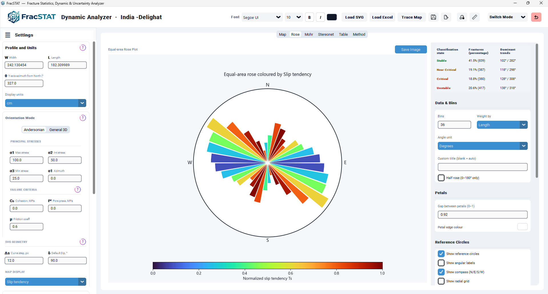
The Rose Tab occupies the full client area of the "Rose" pane in the Dynamic Analyzer's main CTkTabview. Its layout is a two-column CTkFrame grid: a fixed-width plot card on the left (column 0, expandable) containing the Matplotlib canvas, and a fixed-width, vertically scrollable settings panel on the right (column 1, 290 px).
2.1 Plot Card
- Toolbar label — a muted caption reading "Equal-area Rose Plot" identifying the diagram type.
- Save Image button — invokes
self.save_plot_image("rose", self.rose_fig), writing a high-resolution PNG (DPI controlled by the application-wide export setting) to the project'sFracSTAT_plot_exportsfolder. - Polar Matplotlib canvas — a single polar Axes (
self.rose_ax) embedded viaFigureCanvasTkAgg, on which the rose petals, reference circles, compass labels, and title are drawn. - Colour-bar axes — a dedicated, independently positioned Axes (
self.rose_cbar_ax) reserved for the colour scale legend; its rectangle is recomputed on every redraw according to the chosen colour-bar position.
2.2 Settings Panel
The settings panel is a CTkScrollableFrame topped by a fixed fracture-state classification
table (Section 2.2.1) and subdivided below it into five visually separated
cards, each with a bold section header and a thin horizontal rule. Every control is wired
directly to self._draw_rose(), so changes are reflected in the plot immediately
(no separate "Apply" step), with the exception of colour-swatch pickers, which redraw as soon
as a colour is confirmed in the picker dialog.
| Card | Controls contained |
|---|---|
| Data & Bins | Bins, Weight by, Angle unit, Custom title, Half rose toggle |
| Petals | Petal gap fraction, Petal edge colour |
| Reference Circles | Show circles, show angular labels, show compass, show radial grid, circle line width, circle colour |
| Background Colours | Outer (figure) background, inner (axes) background, boundary colour, boundary line width |
| Colour Bar | Position, length fraction, show plot title toggle |
A "Reset to Defaults" button is docked at the bottom of the settings panel and restores every control listed above to its factory value in a single action (see Section 4.7 for the precise reset values, which differ subtly from the tab's initial construction defaults). The classification table is not a user-configurable control and is unaffected by Reset to Defaults; it simply reflects whatever data is currently loaded.
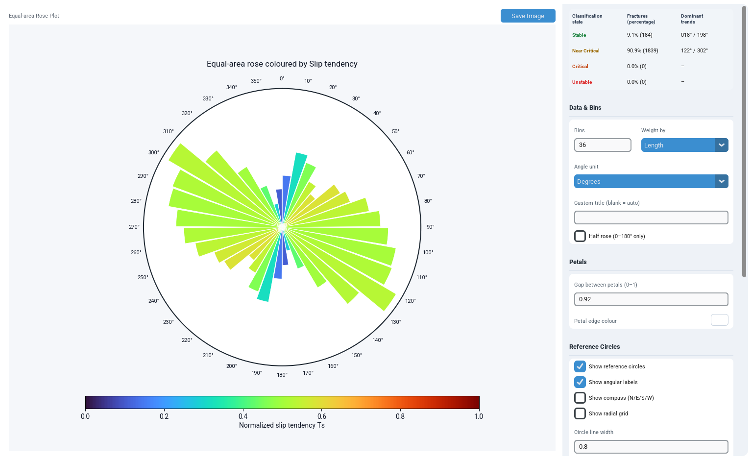
2.2.1 Fracture-State Classification Table
Docked at the very top of the settings panel, above the five cards described in
Section 2.2, is a fixed four-row summary table (built by
_build_rose_classification_table()) with columns "Classification state",
"Fractures (percentage)", and "Dominant trends". Unlike the rest of the settings panel, this
table is not a set of input controls — it is a read-only summary that is refreshed on every
redraw (_update_rose_classification_table(), called from _draw_rose()
with the diagram's current bin count) and is always visible regardless of which Map Display
metric is currently selected for petal colouring.
For each of the four states — Stable, Near Critical, Critical, Unstable, colour-coded to match the palette used elsewhere in the app — the table reports:
- Fractures (percentage) — the count and percentage of all loaded
segments (regardless of orientation) whose
CriticalStatestring column equals that state, e.g. "34.2% (128)". - Dominant trends — among just the segments in that state, the strikes are folded to 0–180° and binned into the same number of angular bins as the current rose diagram; the modal bin's centre and its axial conjugate (offset by 180°) are reported as a "NNN° / NNN°" pair. This identifies which strike orientation is most represented within that risk tier, independent of the strike distribution of the population as a whole. Empty states display "–" in both columns.
Because it is always driven by CriticalState irrespective of the active colouring
metric, this table lets an analyst check the dataset's overall risk profile (e.g. "12% of
fractures are Critical or Unstable, concentrated around 040°/220°") even while the rose
diagram itself is coloured by, say, Slip tendency or Fracture susceptibility.
3. Data Input
The Rose Tab does not load, parse, or import any files itself. It is strictly a consumer of
self.results, the DataFrame produced by core/calculator.py after a
successful Calculate action in the sidebar, or refreshed automatically whenever the stress
parameters, geometry, or dip overrides change. The columns the Rose Tab actually reads are
summarised below.
| Column | Type | Used for |
|---|---|---|
StrikeDeg | float, 0–360° | Base orientation of each segment/plane; folded to 0–180° before binning. |
Length_m | float | Optional length weighting when Weight by = Length. |
| <attribute column> | float or bool | Whichever column self._selected_attribute() resolves to (SlipTendency[Norm], DilationTendency, FractureSusceptibility[Norm], or CriticalStateValue); used to colour each petal. |
3.1 Data Provenance and Column Semantics
StrikeDeg is stored in self.results as a fully-directed 0–360° value
(see models.py's wrap_360 helper) rather than pre-folded to the
0–180° fracture-orientation convention. This design choice is deliberate: preserving the full
compass direction lets the Stereonet and Mohr tabs correctly place a fracture pole on the
correct hemisphere once a per-segment dip override changes the plane from vertical to
inclined. The Rose Tab performs its own fold (StrikeDeg % 180.0) at draw time,
because a rose diagram is inherently an axial (undirected-line) statistic: a joint striking
045° and one striking 225° describe the same physical orientation and must contribute to the
same petal.
Length_m originates from two different geometric pathways depending on the data
source. For SVG-derived segments it is the true, scale-calibrated Euclidean segment length. For
Excel-sourced data without genuine spatial coordinates (legacy fracture-plane tables,
Trend/Plunge pole tables, or focal-mechanism nodal planes) Length_m is populated
with zero for every row unless the source spreadsheet happened to supply an explicit Length
column; see Section 3.2 for how the Rose Tab compensates for this.
3.2 Handling of Missing or Degenerate Length Data
When Weight by = Length is selected but the Length_m column is entirely absent,
all-zero, non-finite, or negative, the module falls back transparently to an equal weight of
1.0 per segment — identical to the Static Analyzer's own Rose Plot tab fallback behaviour (see
the code comment preserved in dynamic_rose_tab.py referencing
static_angles.py). This prevents the diagram from silently rendering as blank when
Excel-sourced orientation-only data (no true geometric length) is loaded, while still weighting
by true length whenever that information genuinely exists.
3.3 Empty-State Handling
If self.results is an empty DataFrame (no segments loaded, or the most recent
Calculate action failed validation), the Rose Tab clears both axes and colour-bar axes and
renders the single caption "No data" in the workspace's muted text colour, then exits without
attempting any further computation. No exception is raised and the settings panel remains
fully interactive so a user can pre-configure display options before data is loaded.
4. Settings and Controls, Card by Card
This section documents every interactive control exposed in the settings panel, in the order
in which it appears, together with its underlying ui_common.qtk variable name, default
value, valid range, and the precise effect on the redraw routine (_draw_rose).
4.1 Data & Bins Card
| Control | Variable | Type / Range | Default | Effect |
|---|---|---|---|---|
| Bins | rose_bins_var | Entry (default 36, range 4–360) | 36 | Number of equal-width angular bins spanning the 0–180° (half rose) or 0–360° (full rose) range. Clamped internally to [4, 360] even if a value were entered programmatically outside the dropdown list. |
| Weight by | rose_weight_var | Dropdown: Length, Count, Equal | Length | Selects the per-segment weight fed into the weighted histogram (see Section 6.2). |
| Angle unit | rose_angle_unit_var | Dropdown: Degrees, Radians, Gradians | Degrees | Controls the numeric format of the angular tick labels only; the underlying binning is always performed in radians and is unaffected. |
| Custom title (blank = auto) | rose_title_var | Free text | "" (empty) | When non-blank and Show plot title is enabled, overrides the automatically generated title string. |
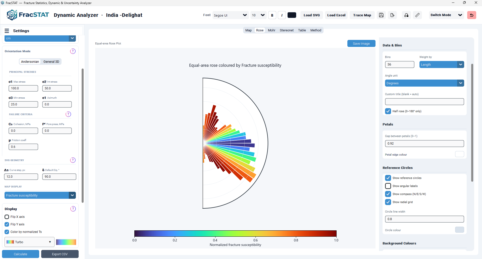
| Half rose (0–180° only) | rose_half_rose_var | Checkbox | Off | Restricts the diagram to a semicircular 0–180° wedge instead of mirroring every strike into both 0–180° and 180–360°. |
4.2 Petals Card
| Control | Variable | Range | Default | Effect |
|---|---|---|---|---|
| Gap between petals (0–1) | rose_petal_gap_var | 0.1–1.0 | 0.92 | Fraction of the full bin angular width actually drawn as the petal's bar width; the remainder appears as whitespace between adjacent petals. A value of 1.0 produces edge-to-edge petals; smaller values increase visual separation. |
| Petal edge colour | rose_petal_edge_color_var | Hex colour | #FFFFFF | Stroke colour applied to every petal's outline (linewidth fixed at 0.6 pt in the drawing routine). |
4.3 Reference Circles Card
| Control | Variable | Type | Default | Effect |
|---|---|---|---|---|
| Show reference circles | rose_show_circles_var | Checkbox | On | Toggles visibility of the polar axes' outer boundary spine (labelled "circles" in the UI, technically the ax.spines['polar'] outline). |
| Show angular labels | rose_show_labels_var | Checkbox | Off | Toggles the numeric/compass tick labels around the circumference. |
| Show compass (N/E/S/W) | rose_show_compass_var | Checkbox | On | Draws bold N/E/S/W text annotations just outside the outermost petal radius; only rendered when the diagram is a full (not half) rose. |
| Show radial grid | rose_show_grid_var | Checkbox | Off | Toggles both the angular and radial (y-axis) gridlines inside the polar plot. |
| Circle line width | rose_circle_lw_var | Numeric text, pt | 0.8 | Line width applied to the radial/angular grid lines when Show radial grid is enabled. |
| Circle colour | rose_circle_color_var | Hex colour | #D9E2EC | Colour applied to the radial/angular grid lines. |
rose_boundary_color_var / rose_boundary_width_var
(Background Colours card), while the internal grid always uses
rose_circle_color_var / rose_circle_lw_var (this card).
4.4 Background Colours Card
| Control | Variable | Type | Default | Effect |
|---|---|---|---|---|
| Outer (figure) background | rose_outer_bg_var | Hex colour | #F5F7FA | Fills the Matplotlib Figure background, i.e. the area outside the circular plot but inside the plot card. |
| Inner (rose) background | rose_inner_bg_var | Hex colour | #FFFFFF | Fills the polar Axes background (the disc enclosed by the outer boundary). |
| Boundary colour | rose_boundary_color_var | Hex colour | #1F2933 | Colour of the polar spine (outer circular boundary), when "Show reference circles" is enabled. |
| Boundary line width | rose_boundary_width_var | Numeric text, pt | 1.5 | Width of the outer boundary spine. |
4.5 Colour Bar Card
| Control | Variable | Type / Range | Default | Effect |
|---|---|---|---|---|
| Position | rose_colorbar_pos_var | Dropdown: Bottom, Top, Left, Right, None | Bottom | Selects which side of the plot the colour-bar legend is docked to, or hides it entirely (None). |
| Length (e.g., 0.72 for 72%) | rose_colorbar_length_var | Numeric text, 0.1–1.0 | 0.72 | Fractional length of the colour bar relative to the available figure dimension along its long axis. |
| Show plot title | rose_show_title_var | Checkbox | On | Toggles rendering of the diagram's title text (auto-generated or custom, per Section 4.1). |
4.6 Colour-by Metric (Controlled Elsewhere)
The Rose Tab does not itself expose a colour-by dropdown; the metric is shared
application-wide with the Map tab via the sidebar's "Map Display" selector
(self.map_mode_var), further modulated by the "Colour by normalized Tₛ" checkbox
(self.normalized_var). The four selectable metrics and their resolved DataFrame
columns are listed below.
| Map Display selection | Normalised? | Resolved column | Colour-bar label |
|---|---|---|---|
| Slip tendency | Yes (default) | SlipTendencyNorm | Normalized slip tendency Tₛ |
| Slip tendency | No | SlipTendency | Slip tendency Tₛ |
| Dilation tendency | n/a | DilationTendency | Dilation tendency Td |
| Fracture susceptibility | Yes | FractureSusceptibilityNorm | Normalized fracture susceptibility (inverted — 1 = least stable; see Section 5.5) |
| Fracture susceptibility | No | FractureSusceptibility | Fracture susceptibility Sf, MPa |
| Critical fractures | n/a | CriticalStateValue | Critical fracture state: 0=Stable, 1=Near Critical, 2=Critical, 3=Unstable |
4.7 Reset to Defaults
The Reset to Defaults button invokes self._rose_reset_defaults(), which writes a
fixed set of values into every control and then calls self._draw_rose(). Two
values differ subtly from the construction-time defaults set by
self._rose_init_vars(): Show angular labels resets to On (constructed default:
Off) and Show radial grid resets to On (constructed default: Off). All other values are
identical between initial construction and reset.
5. Mathematical Background
This section defines, with explicit notation, every quantity computed or displayed by the Rose Tab. Variable names in the source code are given alongside standard geological/statistical symbols where they differ.
5.1 Strike Folding (Axial Data Convention)
A fracture strike is an axial quantity: strikes θ and θ+180° describe the identical line orientation, so the appropriate statistical treatment is that of axial rather than directional data (Mardia and Jupp, 2000). The module therefore folds every strike into the canonical 0–180° domain prior to binning:
where θ_raw is the StrikeDeg column value as stored (0–360°, fully directed). When
the diagram is drawn in full-rose mode (Half rose unchecked), the folded population is mirrored
by adding 180° to obtain a second, duplicate copy, so that the resulting circular histogram
visually fills all four quadrants while still representing purely axial statistics — the
diagram is symmetric about the origin by construction, not because of any new physical
information.
5.2 Weighted Angular Histogram
Let φᵢ be the strike (in radians, after folding and optional mirroring) of segment i, and wᵢ its associated weight (Section 6.2). For a chosen bin count n, the angular domain [0, Φ] — with Φ = π for a half rose or 2π for a full rose — is partitioned into n equal-width bins with edges
The weighted count assigned to bin k is
This is computed via a single call to numpy.histogram with the weights
argument set to the per-segment weight vector
(Harris et al., 2020), which is the standard,
numerically efficient implementation of a weighted circular histogram.
5.3 Equal-Area Petal Radius Transformation
A conventional rose diagram that plots petal radius directly proportional to bin frequency visually over-emphasises the dominant orientation, because the area of a circular sector grows with the square of its radius. FracSTAT follows the standard structural-geology convention of an equal-area (square-root) rose diagram (Fisher, 1993; Davis et al., 2011), in which the plotted radius r_k of each petal is the square root of its weighted count:
Under this transformation, the area of petal k (approximately (1/2)·r_k²·Δθ for narrow bins) becomes directly proportional to C_k, so equal areas on the page correspond to equal frequencies (or equal cumulative lengths, if length-weighted), giving a perceptually honest representation of the underlying distribution and matching the convention used by the Static Analyzer's Rose Plot tab and by widely used structural-geology software.
5.4 Colour-Mapped Attribute Aggregation
Each petal's fill colour represents the mean value of the selected mechanical attribute A (one of Tₛ (Morris et al., 1996), Td (Ferrill and Morris, 2003), Sf (Streit and Hillis, 2004), or the four-tier critical-fracture-state value) among all segments falling in that bin:
If a bin contains no segments, Ā_k defaults to 0.0 rather than NaN, which prevents matplotlib
colour-mapping errors for empty angular sectors. The colour scale and normalisation strategy
applied to Ā_k are delegated to self.attribute_colormap_and_norm(), the same
routine used by the Map and Mohr tabs, ensuring colour consistency across the whole Dynamic
Analyzer workspace (see Section 5.5).
5.5 Normalisation Strategy
Continuous attributes (SlipTendency, SlipTendencyNorm, DilationTendency,
FractureSusceptibility, FractureSusceptibilityNorm) are mapped through a standard linear
Normalize instance. Columns whose name ends in "Norm", together with DilationTendency,
are fixed to the domain [0, 1]; all other continuous columns use the
finite data-driven minimum and maximum, with a small symmetric padding applied when the data
range collapses to a single value (to avoid a degenerate colour scale). Note that
FractureSusceptibilityNorm is inverted at source in
core/calculator.py — 1 − (S_f − min) / (max − min) —
because a lower S_f means a smaller remaining pore-pressure margin; on this tab that means a
petal at the top of the [0, 1] colour domain contains the least stable fractures, and
the scale is relative to the loaded dataset rather than to a failure threshold. The
CriticalStateValue attribute instead uses a discrete four-colour colormap/norm banding its
integer codes 0–3 (Stable, Near Critical, Critical, Unstable), guaranteeing that each
state maps unambiguously to its own flat colour swatch rather than a continuous gradient, and
the colour bar in this special case is manually re-ticked to read "Stable" / "Near Critical" /
"Critical" / "Unstable" instead of numeric values. Because each petal's colour value Ā_k is a
mean of the per-segment state codes in that bin (Section 5.4), a
petal spanning a mix of states can render at a boundary or blended position on the discrete
scale rather than falling cleanly into a single band.
6. Algorithms
6.1 Bin Count Resolution and Sanitisation
The bin-count text is parsed with a defensive try/except around int(); a parse
failure falls back silently to 36. The resulting integer is clamped to the closed interval
[4, 360] via max(4, min(360, n)), guarding against pathological inputs (e.g., a
bin count of 0 that would crash numpy.histogram, or an excessively large value
that would render an unreadably dense diagram).
6.2 Weight Vector Construction
| Mode | Weight construction | Fallback condition |
|---|---|---|
| Length | w_i = Length_m_i (metres, or the active display unit) | If Length_m is absent, or every value is non-finite/≤0, w_i = 1.0 for all i (equal weighting). |
| Count | w_i = 1.0 | None — always uniform. |
| Equal | w_i = 1.0 | None — identical numerical result to Count in the current implementation. |
6.3 Mirroring for Full-Rose Display
When Half rose is unchecked, the strike array and its weight array are each duplicated: the
mirrored strike array is np.concatenate([strikes, strikes + 180]), and the
mirrored weight array is np.tile(weights, 2). The colour-attribute array is
likewise duplicated with np.tile so that every mirrored strike sample still
carries its correct source attribute value into the per-bin colour-averaging step.
6.4 Petal Geometry Assembly
- Compute bin edges over [0, Φ] for n bins; derive bin centres and widths.
- Compute the weighted histogram C_k over the (possibly mirrored) strike population.
- Compute equal-area radii r_k = √C_k.
- For each bin, gather the subset of attribute values whose strike falls in [e_k, e_(k+1)) and take the mean (0.0 if empty) to obtain the per-petal colour value Ā_k.
- Resolve (colormap, norm, is_critical) from
self.attribute_colormap_and_norm(Ā, value_column). - Map Ā through a ScalarMappable to obtain an RGBA colour array, one entry per bin.
- Draw all bins in a single
ax.bar(...)call with theta = bin centres, height = r_k, width = (bin width) × petal-gap fraction, and per-bin RGBA facecolor.
strikes_deg = self.results["StrikeDeg"].to_numpy(dtype=float) % 180.0
if half:
    strikes_full = strikes_deg
    weights = raw_weights
else:
    strikes_full = np.concatenate([strikes_deg, strikes_deg + 180.0])
    weights = np.tile(raw_weights, 2)

strikes = np.deg2rad(strikes_full)
bins = np.linspace(0.0, full_range, num_bins + 1)
counts, edges = np.histogram(strikes, bins=bins, weights=weights)
centers = (edges[:-1] + edges[1:]) / 2.0
widths = np.diff(edges)

# per-bin mean attribute value -> petal colour
color_values = []
for low, high in zip(edges[:-1], edges[1:]):
    mask = (strikes >= low) & (strikes < high)
    color_values.append(
        float(np.nanmean(attribute_values[mask])) if mask.any() else 0.0
    )
color_values = np.array(color_values)
Simplified excerpt of _draw_rose() showing the strike-folding, mirroring, weighted-histogram, and per-bin colour-aggregation steps.
6.5 Angular Tick-Label Generation
Tick positions are always generated at a fixed 10° cadence in the underlying degree domain
(np.arange(0, 360, 10)), regardless of the display unit chosen. The three
supported unit modes reformat the same tick positions rather than recomputing them:
| Unit mode | Tick spacing used for labels | Label format |
|---|---|---|
| Degrees | 10° (0, 10, 20, …, 350) | "{n}°" |
| Radians | 30° (0, 30, …, 330) | Multiples of π expressed as a decimal fraction, e.g. "0.33π"; the origin is rendered as "0" |
| Gradians | 10° (0, 10, …, 350) | Degrees converted via g = d × 400/360 and rendered as "{g}g" |
6.6 Colour-Bar Layout Algorithm
Because the colour bar can be docked to any of four sides (or hidden), the module maintains four hard-coded layout presets, each specifying (a) the [x0, y0, width, height] rectangle (figure-fraction coordinates) for the dedicated colour-bar Axes, and (b) a corresponding rectangle that the polar Axes itself is resized/repositioned into so the two never overlap. The presets are summarised below (all values are matplotlib figure-fraction coordinates, i.e. 0–1).
| Position | Colour-bar rectangle [x0, y0, w, h] | Polar-axes rectangle [x0, y0, w, h] | Orientation |
|---|---|---|---|
| Bottom | [(1−L)/2, 0.06, L, 0.030] | [0.15, 0.20, 0.70, 0.65] | Horizontal |
| Top | [(1−L)/2, 0.92, L, 0.030] | [0.15, 0.10, 0.70, 0.65] | Horizontal |
| Left | [0.03, (1−L)/2, 0.025, L] | [0.18, 0.15, 0.70, 0.70] | Vertical |
| Right | [0.93, (1−L)/2, 0.025, L] | [0.10, 0.15, 0.70, 0.70] | Vertical |
| None | (hidden) | [0.15, 0.12, 0.70, 0.75] | n/a |
L denotes the user-supplied colour-bar length fraction (rose_colorbar_length_var),
clamped to [0.1, 1.0]. This deterministic, closed-form layout avoids the layout-engine
recomputation cost of matplotlib's constrained_layout on every redraw and
guarantees pixel-stable behaviour when a user resizes the colour bar interactively.
7. Internal Workflow
This section summarises the end-to-end control flow triggered whenever the Rose Tab must be (re)drawn — on initial tab construction, whenever a setting changes, whenever new stress results are calculated, and whenever a fracture segment is selected/deselected elsewhere in the workspace.
7.1 Construction Sequence
SlipTendencyApp._build_layout()callsself._build_rose_tab()once, during workspace initialisation._build_rose_tab()callsself._rose_init_vars()to lazily create every CTk variable (usinghasattrguards so repeated calls are idempotent).- The plot card, toolbar, Matplotlib Figure/Axes/canvas, and dedicated colour-bar Axes are instantiated and gridded.
self._build_rose_settings_panel(tab)constructs the five-card scrollable settings panel and wires every widget's command/binding toself._draw_rose(or, for text-entry fields, to the widget's<Return>and<FocusOut>events).- No explicit initial draw call occurs inside
_build_rose_tab(); the first paint happens the moment the sharedrefresh_plots()/calculate()pipeline (indynamic_app.py) subsequently invokesself._draw_rose()once data becomes available, or via the workspace's periodic full-refresh path.
7.2 Redraw Sequence (_draw_rose)
- Guard clause: if
self.rose_axhas not yet been created, return immediately (defensive check for calls that may race construction). - Read the background, edge, and circle colour values from their StringVars.
- Clear both the polar Axes and the colour-bar Axes; hide the colour-bar Axes pending recomputation; apply the outer and inner background colours to the Figure and Axes respectively.
- If
self.resultsis empty, render the "No data" caption and return. - Parse and clamp the bin count.
- Resolve the half/full-rose flag and the corresponding angular domain Φ.
- Build the weight vector per Section 6.2.
- Fold StrikeDeg into 0–180°; mirror strikes/weights into 0–360° if a full rose is requested.
- Compute the weighted histogram and equal-area radii.
- Resolve the active colour-by attribute via
self._selected_attribute(); tile the attribute array to match any mirroring; compute per-bin mean attribute values. - Resolve (cmap, norm, is_critical) via
self.attribute_colormap_and_norm()and map to an RGBA array. - Parse and clamp the petal-gap fraction; draw all petals in one
ax.bar()call. - Configure polar orientation (theta zero at North, clockwise direction, half/full theta limits).
- Parse the circle line width; compute and apply angular tick positions/labels per the selected unit, or clear tick labels if disabled.
- Apply boundary spine visibility/colour/width; apply internal grid visibility/colour/width; hide radial (r-axis) tick labels unconditionally.
- If compass labels are enabled and the rose is a full rose, annotate N/E/S/W at 1.10× the maximum petal radius.
- If the title is enabled, compute the auto title string (or use the custom override) and apply it, sized from the current global font-size rcParam.
- Parse and clamp the colour-bar length; select and apply the layout preset from Section 6.6, or hide the colour bar and expand the polar Axes to fill the card if Position = None.
- Call
self.rose_canvas.draw_idle()to schedule an asynchronous repaint.
7.3 Cross-Tab Interactions
The Rose Tab is a passive consumer within the broader workspace: it exposes no
segment-selection or picking behaviour of its own (unlike the Map, Mohr, and Stereonet tabs,
which support click-to-select and cross-tab highlighting). It is, however, refreshed
automatically whenever refresh_plots() is invoked following a Calculate action, a
colour-scale change, a stress-parameter edit, a dip-override load, or a global font/appearance
change (via _apply_workspace_font, which forces a redraw of every plot so that
title and label font sizes stay in sync with the header's Font Size control).
8. Statistical Methods
8.1 Circular (Directional) Statistics Context
The rose diagram is fundamentally a graphical circular-statistics device for axial data (Mardia and Jupp, 2000; Fisher, 1993), and is standard structural-geology practice (Davis et al., 2011). Because fracture strikes are axial (mod 180°) rather than directional (mod 360°) quantities, the folding and mirroring steps described in Section 5.1 are essential; failing to fold strikes before binning would artificially split a genuinely unimodal fracture set into two half-populations 180° apart.
8.2 Weighted Frequency vs. Length-Weighted Intensity
Selecting Weight by = Length converts the diagram from a simple strike-frequency histogram (each fracture contributes equally regardless of size) into a length-weighted orientation histogram, which more closely approximates the areal or volumetric fracture intensity contributed by each strike set — a metric of direct relevance to fluid-flow anisotropy and fracture-network connectivity assessments. Selecting Count or Equal instead answers a purely frequency-based question ("how many fractures strike in this direction"), which is less sensitive to a small number of unusually long fractures dominating the diagram.
8.3 Per-Bin Attribute Aggregation as a Simple Statistical Estimator
The colour value assigned to each petal, Ā_k (Section 5.4), is an unweighted arithmetic mean of the selected mechanical attribute over all segments in that bin — it is not weighted by the same length/count weighting used for the petal radius. Analysts should therefore interpret petal colour as "the typical stress-attribute value among fractures at this orientation" and petal size as "how much of the population (by count or length) occurs at this orientation"; the two encodings answer distinct statistical questions and are not meant to be multiplied together to recover a single combined score.
8.4 Handling of Empty Bins
Bins containing zero segments are assigned Ā_k = 0.0, and will typically render as either the coolest end of the active colormap or, for the critical-fracture-state metric, the "Stable" colour swatch. Users comparing colour intensity across bins with very different populations (e.g., a dominant fracture set with hundreds of members versus a minor set with two or three) should cross-reference petal length before drawing mechanical conclusions from colour alone, since a small-n bin's mean attribute value is a comparatively unstable estimator.
9. Visualization Components
9.1 Polar Coordinate Convention
The Axes is configured with theta_zero_location = 'N' (0° at the top of the plot,
matching geographic North) and theta_direction = -1 (clockwise increasing angle),
reproducing the standard geological compass-bearing convention rather than matplotlib's
mathematical default (0° at east, counter-clockwise).
9.2 Petal Rendering
All petals are drawn with a single vectorised ax.bar(theta, radius, width, bottom=0,
color=..., edgecolor=..., linewidth=0.6) call rather than one bar() call
per bin, which is significantly faster for large bin counts and produces a single collection of
matplotlib artists that is easier to manage across repeated redraws.
9.3 Reference Geometry
- Outer boundary spine — the polar plot's circular frame, colour/width controlled by the Background Colours card, visibility by the Reference Circles card's "Show reference circles" toggle.
- Internal angular/radial grid — matplotlib's native polar grid, colour/width from the Reference Circles card, visibility from "Show radial grid".
- Compass annotations — bold N/E/S/W text placed at 1.10× the maximum bar radius, shown only for full (not half) roses.
9.4 Colour Bar
The colour bar is a standard matplotlib Colorbar object bound to the ScalarMappable created from the resolved colormap and norm. For the CriticalStateValue metric, its ticks are explicitly overridden to the four labelled positions [0, 1, 2, 3] with text labels "Stable", "Near Critical", "Critical", and "Unstable" rather than a numeric scale, which is essential because the underlying discrete norm would otherwise present as a continuous-looking gradient despite representing a fixed four-state classification.
9.5 Title
When enabled, the title reads either the user-supplied custom string, or the automatically
generated string "Equal-area rose coloured by {value_title}", where value_title is the third
element of the tuple returned by self._selected_attribute() (e.g., "Slip
tendency", "Dilation tendency"). Title font size is drawn from matplotlib's live
axes.titlesize rcParam, which is itself kept synchronised with the workspace
header's Font Size control by _apply_workspace_font, so all diagrams across the
Dynamic Analyzer scale their text together.
10. Advanced Features
10.1 Synchronised Colour Semantics Across Tabs
Because self.attribute_colormap_and_norm() and self._selected_attribute()
are shared, application-level methods rather than Rose-Tab-local logic, changing the Map
Display metric or the active colormap in the sidebar simultaneously updates the Map tab, the
Rose tab, and (for the continuous metrics) the Mohr tab's colour field, guaranteeing that a
given colour always represents the same numeric value everywhere in the workspace during a
single analysis session.
10.2 Unit-Agnostic Length Weighting
The Length_m column already reflects the workspace's active display unit
conversion pipeline (the profile width/height and unit selector in the sidebar), so switching
the display unit (m, cm, mm, km) does not require any additional handling inside the Rose Tab
— the weighted histogram automatically reflects lengths in whichever unit is currently active,
though the colour-bar and axis labels for the rose diagram itself carry no unit text since the
y-axis (radius) has no numeric meaning beyond relative area.
10.3 Interactive Colour Pickers
Every colour field in the settings panel uses the shared _StaticColorButton
widget (ui_widgets.py), which opens a 40-swatch preset palette (5 shade rows × 8
hues) plus a free-form hex-code entry with a live preview swatch. Selecting or confirming a
colour immediately triggers self._draw_rose() via the widget's callback, and the
corresponding StringVar is kept in sync via a trace_add('write', ...) binding so
the swatch button visually reflects the underlying variable's current value even if it is
changed programmatically (e.g., by Reset to Defaults).
10.4 Dynamic Font Scaling
Font sizes for the title, tick labels, and colour-bar text are never hard-coded; they are read
live from matplotlib's global rcParams (axes.titlesize, xtick.labelsize)
at draw time, which are themselves driven by the workspace header's Font, Font Size, Bold, and
Colour controls. This design keeps every plot in the Dynamic Analyzer — Map, Rose, Mohr,
Stereonet — visually consistent without requiring the Rose Tab to know about the header's
implementation.
11. Performance Optimization
| Technique | Where applied | Benefit |
|---|---|---|
| Vectorised NumPy histogram | Section 6.2/6.4, np.histogram(weights=...) | O(n) weighted binning without an explicit Python loop over segments. |
Single ax.bar() call for all petals | Section 9.2 | Avoids per-bin matplotlib artist creation overhead; scales to the maximum supported 360 bins without perceptible lag. |
draw_idle() rather than draw() | End of _draw_rose | Defers the actual canvas repaint to Qt's event loop, coalescing rapid successive setting changes (e.g., a slider or rapid typing) into fewer physical repaints. |
| Deterministic closed-form colour-bar layout | Section 6.6 | Avoids the per-frame cost of matplotlib's automatic constrained/tight layout solvers. |
| Idempotent variable initialisation | Section 7.1, hasattr guards in _rose_init_vars | Prevents redundant variable churn if the tab-build path is ever invoked more than once. |
| Shared colormap/normalisation resolution | Section 10.1 | Colour-scale computation logic lives in one place (SlipTendencyApp) rather than being duplicated per tab, reducing both code size and the chance of visual inconsistency. |
No caching layer is applied to the Rose Tab's own computation, because the weighted-histogram
and colour-aggregation steps are computationally inexpensive (typically well under a few
milliseconds for datasets of several thousand segments) relative to the cost of a full stress
recalculation (core/calculator.py) or a Matplotlib canvas repaint; the module
instead relies on the shared workspace-level dirty-tracking (self._ws_mark_dirty())
and on-demand redraw pattern common to all Dynamic Analyzer tabs.
12. Practical Examples
12.1 Example 1 — Identifying the Dominant, Critically-Stressed Fracture Set
- Load an SVG trace map or Excel orientation table and click Calculate with a representative in-situ stress tensor.
- In the sidebar, set Map Display to "Critical fractures".
- Switch to the Rose tab; set Weight by = Length and Bins = 36 for a balanced angular resolution.
- Observe which petal(s) are both large (abundant/long fractures at that strike) and coloured with the "Critical" or "Unstable" swatch — these represent the strike orientations most likely to be actively slipping or on the verge of Coulomb failure under the assumed stress state.
12.2 Example 2 — Comparing Frequency- vs. Length-Weighted Orientation Distributions
- Draw the rose with Weight by = Count to see which strike bins contain the most individual fracture segments.
- Redraw with Weight by = Length; note any change in the dominant petal — a strike bin with few but very long fractures may become dominant under length weighting even though it was subordinate under count weighting.
- Use this comparison to decide whether a proposed fracture set is genuinely volumetrically significant or is merely numerically prevalent due to digitisation of many short segments.
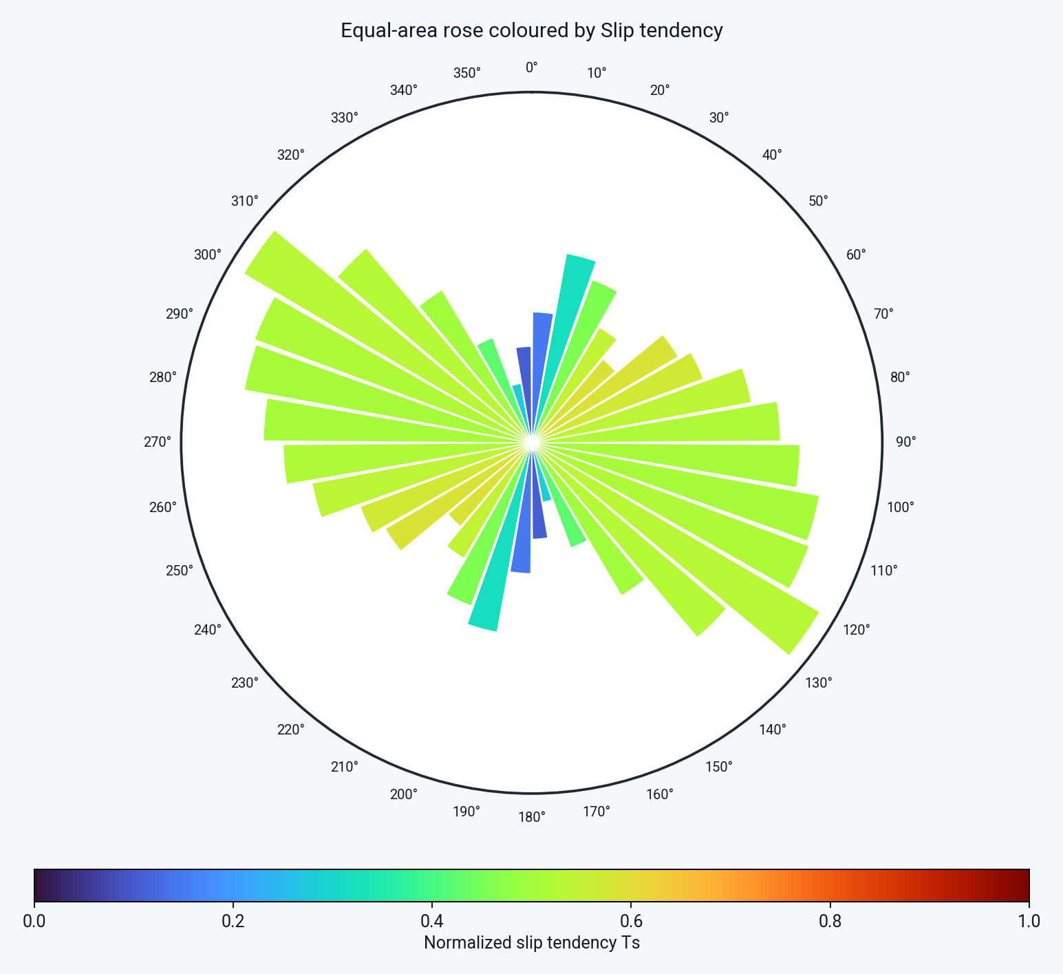
12.3 Example 3 — Publication-Quality Export
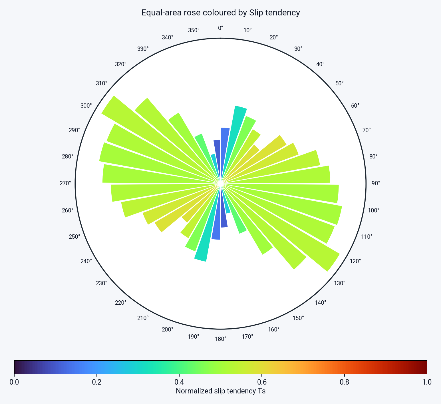
- Set the desired custom title via the Custom title field (e.g., "Well A-1 — Fracture Rose Coloured by Normalized Slip Tendency").
- Adjust Outer/Inner background colours, boundary width, and petal edge colour to match the target journal's figure style.
- Set Colour Bar → Position to Right and Length to approximately 0.6 for a compact vertical legend suitable for a two-column layout.
- Click Save Image; the resulting PNG is written at the application-configured export DPI to the project's
FracSTAT_plot_exportsdirectory, ready for direct inclusion in a manuscript or report.
13. Geological Interpretation
The Rose Tab's combined orientation/mechanics encoding directly supports several core geomechanical workflows in fracture-network characterisation and reservoir/rock-slope stability analysis.
13.1 Reactivation-Prone Set Identification
Under Andersonian faulting theory (Anderson, 1951), fractures oriented at the Coulomb-optimal angle to σ1 (approximately 2θ_opt = arctan(1/μ) from σ1, i.e. roughly 25°–35° for typical friction coefficients) exhibit the highest ratio of shear to effective normal stress and are therefore the most prone to frictional reactivation (Jaeger et al., 2007). A petal that is both prominent (high frequency or cumulative length) and coloured toward high slip tendency or the "Critical"/"Unstable" classification at approximately this optimal angular offset is a strong candidate for active or potentially active slip under the assumed stress state (Morris et al., 1996).
13.2 Dilation and Fluid-Flow Pathways
When Map Display is set to Dilation tendency, petals coloured toward high Td highlight strike sets that are mechanically favoured to open (dilate) rather than shear under the current stress field — these orientations are of particular interest for identifying preferential fluid-flow pathways or high-permeability fracture corridors in naturally fractured reservoirs, since dilated fractures typically exhibit enhanced hydraulic aperture relative to shear-dominated sets (Ferrill and Morris, 2003; Zoback, 2007).
13.3 Fracture Susceptibility as a Composite Risk Indicator
Fracture susceptibility Sf combines the normal-stress clamping effect, pore pressure, cohesion, and friction into a single margin-to-failure metric (see Section 5 of the Method tab documentation for the full formula), read most naturally as the pore-pressure increase a plane can tolerate before it slips (Streit and Hillis, 2004). Colouring the rose by susceptibility allows an analyst to rank strike sets by their overall geomechanical risk in a single view, complementing the four-tier Critical fractures classification with a continuous gradation useful for sensitivity or what-if stress-scenario comparisons.
13.4 Comparing Geometric vs. Mechanical Fabric
Because the Static Analyzer's own Rose Plot tab depicts the same fracture population's purely geometric strike distribution (uncoloured by any stress attribute), a useful diagnostic workflow is to compare the Static Analyzer's rose against the Dynamic Analyzer's stress-coloured rose for the same dataset: strike sets that are geometrically minor but mechanically critical may represent an under-sampled but geomechanically important fracture population warranting additional field verification or targeted sampling.
14. Implementation Notes
14.1 Class and File Organisation
RoseTab is implemented as a Python mixin class (no independent __init__
or base class of its own) intended solely to be combined via multiple inheritance into
SlipTendencyApp alongside MapTab, MohrTab,
TableTab, MethodTab, and StereonetTab. This mixin pattern
is used consistently throughout FracSTAT's Dynamic and Static Analyzer workspaces to keep each
tab's construction and drawing logic in its own source file while sharing a single top-level
application-state object.
14.2 Variable Naming Convention
Every ui_common.qtk variable owned by this tab is prefixed rose_ (e.g.,
rose_bins_var, rose_show_circles_var) to avoid collisions with the
many other tabs' variables that coexist on the same SlipTendencyApp instance.
14.3 Defensive Parsing
All free-text numeric entries (bin count, petal gap, circle line width, σ1 line width, colour-bar length, boundary width) are parsed with a try/except ValueError pattern that falls back to a hard-coded sane default rather than raising an exception into the Qt event loop, ensuring the application never crashes from a malformed or empty text entry.
14.4 Unused Helper Function
The module defines a small utility, _hex_to_rgb01(hex_color), which converts a
'#RRGGBB' string into a normalised (r, g, b) tuple in the [0, 1] range. This helper is not
currently invoked anywhere within the drawing pipeline (all colour handling is delegated to
matplotlib's native hex-colour support) and is retained in the source as a utility available
for any future feature requiring raw RGB tuples.
14.5 Dependency Summary
| Library | Role |
|---|---|
numpy | Weighted histogram binning, angular array manipulation, trigonometric conversions. |
matplotlib (pyplot Figure/Axes API) | Polar plot rendering, colour mapping (ScalarMappable), colour-bar construction. |
matplotlib.backends.backend_qtagg | Embeds the Matplotlib Figure inside the Qt canvas widget (FigureCanvasTkAgg, the ui_common.qtk shim over FigureCanvasQTAgg). |
ui_common.qtk (ctk) | All settings-panel widgets: frames, labels, entries, checkboxes, option menus, buttons. |
ui_common.ui_widgets | Supplies _StaticColorButton, the shared swatch/hex colour-picker widget. |
15. Limitations
| Limitation | Description |
|---|---|
| Unweighted colour aggregation | Per-bin colour aggregation uses a simple arithmetic mean with no weighting by segment length or count, which can make small-population bins visually as prominent in colour intensity as large, statistically robust bins; users must cross-reference petal size when interpreting colour. |
| Compass labels tied to Half rose toggle | The compass N/E/S/W annotations are suppressed for half-rose diagrams, which is an intentional design choice (the half rose only spans 0–180° and W/S annotations would be geometrically meaningless in that mode), but is not configurable independently of the Half rose toggle. |
| No orientation-bias correction | Every fracture contributes with equal weight regardless of the angle at which the sampling line or outcrop face intersects it, so sets sub-parallel to the sampling direction are systematically under-represented. No Terzaghi weighting is applied (Terzaghi, 1965). |
| No circular summary statistics or significance tests | The tab is purely graphical: it reports no mean strike, resultant length, circular variance, or test of uniformity, all of which would be needed to state whether an apparent preferred orientation is statistically significant (Mardia and Jupp, 2000; Fisher, 1993). |
| Bin count is a free parameter | Petal count is set by hand with no data-driven rule. Because a rose diagram's apparent modality can change materially with bin width, the chosen bin count should always be reported and ideally varied to confirm that a peak is robust (Fisher, 1993). |
| Strike only, dip discarded | Folding to a 0–180° strike domain (Section 5.1) collapses the full three-dimensional plane orientation onto a single azimuth, so two sets sharing a strike but dipping oppositely are indistinguishable here. Use the Stereonet tab where dip matters (Davis et al., 2011). |
| Colour scale is dataset-relative for susceptibility | FractureSusceptibilityNorm is rescaled and inverted against the loaded file's own minimum and maximum (Section 5.5), so a saturated petal marks the least stable orientation in that file, not one at failure. Values are not comparable between datasets. |
16. References
Sources are listed alphabetically within each group. In-text citations throughout this page link to the corresponding entry below.
16.1 Circular and Directional Statistics
- Fisher, N. I. (1993). Statistical Analysis of Circular Data. Cambridge University Press. https://doi.org/10.1017/CBO9780511564345
- Mardia, K. V., & Jupp, P. E. (2000). Directional Statistics. John Wiley & Sons, Chichester. https://doi.org/10.1002/9780470316979
- Terzaghi, R. D. (1965). Sources of error in joint surveys. Géotechnique, 15(3), 287–304. https://doi.org/10.1680/geot.1965.15.3.287
16.2 Structural Geology, Stress and Reactivation
- Anderson, E. M. (1951). The Dynamics of Faulting and Dyke Formation with Applications to Britain (2nd ed.). Oliver and Boyd, Edinburgh.
- Davis, G. H., Reynolds, S. J., & Kluth, C. F. (2011). Structural Geology of Rocks and Regions (3rd ed.). John Wiley & Sons. ISBN 978-0-471-15231-6.
- Ferrill, D. A., & Morris, A. P. (2003). Dilational normal faults. Journal of Structural Geology, 25(2), 183–196. https://doi.org/10.1016/S0191-8141(02)00029-9
- Jaeger, J. C., Cook, N. G. W., & Zimmerman, R. W. (2007). Fundamentals of Rock Mechanics (4th ed.). Blackwell Publishing, Oxford. ISBN 978-0-632-05759-7.
- Morris, A., Ferrill, D. A., & Henderson, D. B. (1996). Slip-tendency analysis and fault reactivation. Geology, 24(3), 275–278. https://doi.org/10.1130/0091-7613(1996)024<0275:STAAFR>2.3.CO;2
- Streit, J. E., & Hillis, R. R. (2004). Estimating fault stability and sustainable fluid pressures for underground storage of CO₂ in porous rock. Energy, 29(9–10), 1445–1456. https://doi.org/10.1016/j.energy.2004.03.078
- Zoback, M. D. (2007). Reservoir Geomechanics. Cambridge University Press. https://doi.org/10.1017/CBO9780511586477
16.3 Software
- Harris, C. R., Millman, K. J., van der Walt, S. J., Gommers, R., Virtanen, P., Cournapeau, D., … Oliphant, T. E. (2020). Array programming with NumPy. Nature, 585(7825), 357–362. https://doi.org/10.1038/s41586-020-2649-2
- Hunter, J. D. (2007). Matplotlib: A 2D graphics environment. Computing in Science & Engineering, 9(3), 90–95. https://doi.org/10.1109/MCSE.2007.55
Methods statement for the Rose Tab. If a figure produced by this tab appears in a publication, the details below are what a reader needs in order to reproduce it, and are what the citations above assume:
Equal-area (square-root radius) rose diagram of fracture strike, folded to the 0–180° axial domain (Mardia and Jupp, 2000), computed with B equal-width bins and weighted by trace length (or by count, as stated) from n observations, drawn as a half or mirrored full rose as stated. Petals coloured by the bin-mean value of the selected stress-tendency metric — slip tendency (Morris et al., 1996), dilation tendency (Ferrill and Morris, 2003), fracture susceptibility (Streit and Hillis, 2004), or the four-tier critical-state code — for σ₁/σ₂/σ₃ = … MPa, P_f = … MPa, C₀ = … MPa and μ = … (Jaeger et al., 2007). Implemented in NumPy (Harris et al., 2020) and rendered with Matplotlib (Hunter, 2007). Report B, n, the weighting mode, the stress tensor, and the colour metric; note that petal colour is an unweighted bin mean (Section 8.3) and that no orientation-bias correction is applied (Section 15).