Dynamic Method Tab
Located at dynamic_analyzer/tabs/dynamic_method_tab.py, the Method
tab (implemented as the mixin class MethodTab) is the Dynamic Analyzer's built-in,
read-only reference sheet. Unlike every other tab in the Dynamic Analyzer, it consumes no
project data and produces no plot — it exists purely to document, in one place, the exact
geometric and stress-mechanical formulas that the Map, Rose, Mohr, and Table tabs apply to every
loaded fracture segment. It is the single source of truth a user can check to confirm precisely
how a reported stress angle, slip tendency, or Coulomb failure state was derived.
On this page
1. Interface Overview
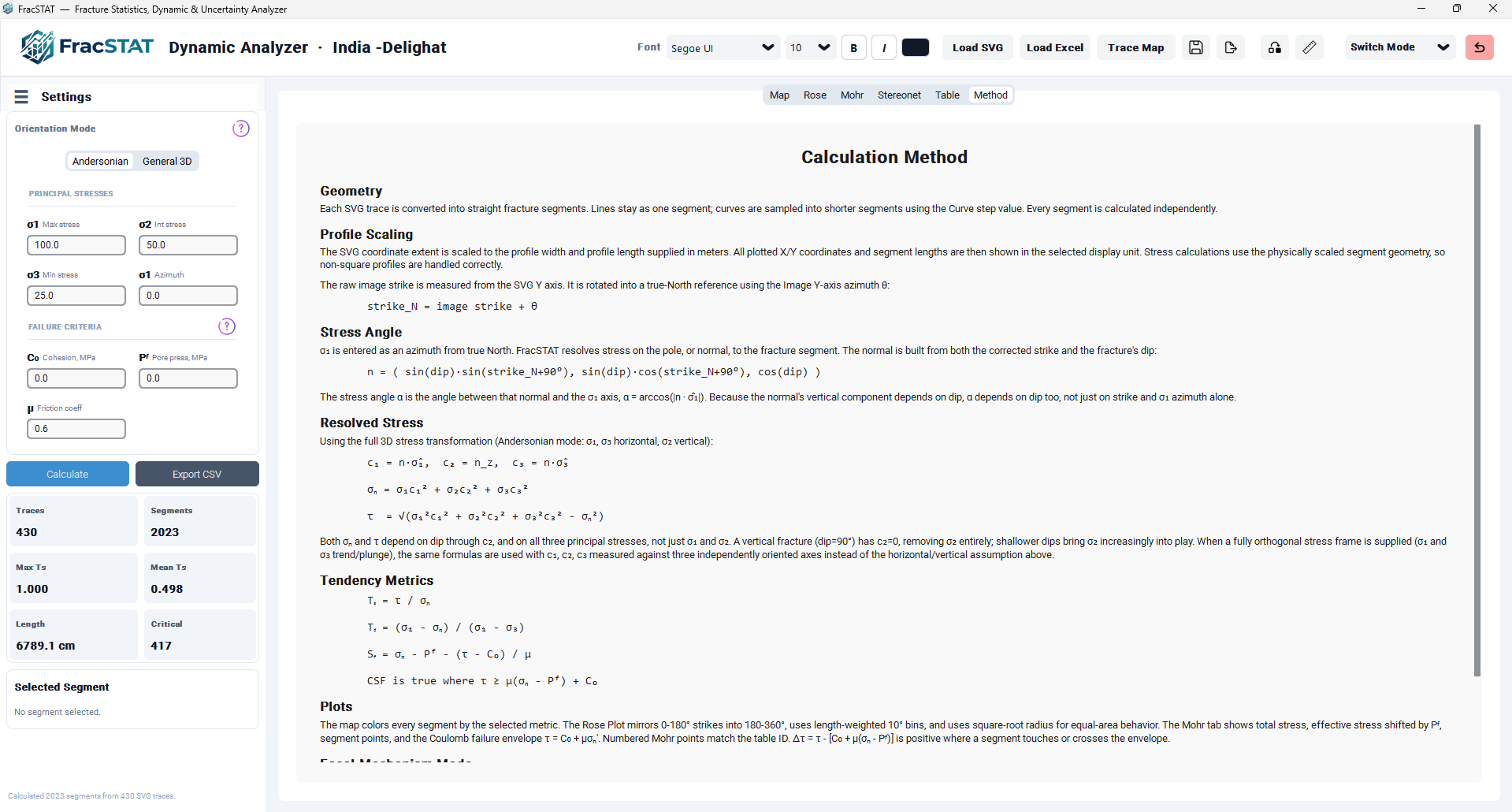
The Method tab occupies the full width of its workspace tab with a single scrollable
CTkTextbox widget, padded 20 px on every side to give the text a clean,
card-like appearance. There is no sidebar, no plot canvas, and no interactive control of any
kind — the widget is explicitly locked to a read-only (state="disabled") state
immediately after its content is inserted, so the tab behaves purely as documentation rendered
inside the application itself rather than as an analysis surface.
2. Purpose and Scope
Every other tab in the Dynamic Analyzer — Map, Rose, Mohr, Stereonet, and Table — resolves stress onto fracture planes and reports derived quantities such as slip tendency, dilation tendency, susceptibility, and Coulomb failure state, but none of them re-explain the underlying formulas at the point of use. The Method tab exists to close that gap: it is a static, in-application reference that a user can open at any time to see, in order, exactly how raw SVG geometry is turned into a scaled fracture network, how that network's strikes are corrected to true North, how the stress angle to each fracture is computed, how normal and shear stress are resolved via the 2-D Mohr transformation, and how each of the tendency and failure metrics reported elsewhere in the workspace is defined.
Because the tab performs no calculation of its own — it only documents calculations performed
by other tabs — it has no data-input requirements, no settings, and no redraw logic. Its entire
behaviour is determined once, at tab-build time, by the sequence of text.insert()
calls in _build_method_tab().
3. Content Structure and Typography
The tab uses the ui_common.qtk text-widget tag API to give the reference sheet a typographic hierarchy
without resorting to a rich-text or HTML rendering engine. Four fonts and five tags are defined
once at build time and then applied selectively as each line is inserted.
| Tag | Font | Role |
|---|---|---|
title | Roboto, 22 pt, bold, centred | The single page heading, "Calculation Method". |
header | Roboto, 16 pt, bold | Section headings (Geometry, Profile Scaling, Stress Angle, Resolved Stress, Tendency Metrics, Plots, Focal-Mechanism Mode). |
body | Roboto, 13 pt, regular | Explanatory prose beneath each section heading. |
math | Consolas, 14 pt monospace, left-indented | Inline formula lines, indented 30 px from both margins for visual separation from prose. |
sub | Consolas, 10 pt monospace, vertical offset −4 px | Combined with math to render a subscripted symbol (e.g. the "s" in Ts) at reduced size and lowered baseline within an otherwise monospaced formula line. |
CTkTextbox cannot mix a smaller, baseline-shifted
run of characters into the middle of a single inserted string, every subscripted symbol used in
the Tendency Metrics section (Ts, Td, Sf) is built from three
separate insert() calls — the base letter tagged math, the subscript
character tagged with the combined ("math", "sub") tuple, and the remainder of the
formula tagged math again — rather than from one call carrying the whole line.
4. Mathematical Background
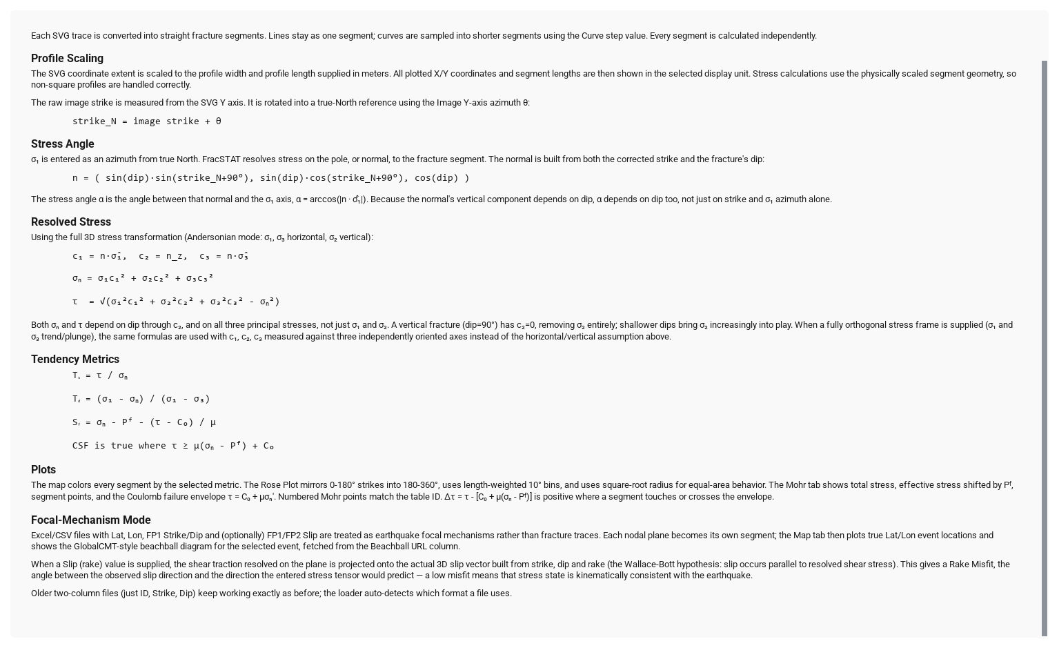
The reference sheet proceeds through five formula-bearing sections, in the same order every other Dynamic Analyzer tab implicitly relies on: geometry construction, profile scaling and strike correction, the stress angle definition, the resolved-stress transformation, and the tendency/failure metrics computed from that resolved stress.
4.1 Geometry
Every digitised SVG trace is converted into one or more straight fracture segments before any stress calculation begins. A line primitive in the source SVG becomes exactly one segment; curved primitives are sampled into a series of shorter straight segments according to the workspace's Curve step setting, exactly mirroring the tessellation approach used by the Static Analyzer's geometry engine. Every resulting segment — whether from an originally straight or originally curved trace — is treated identically and calculated independently by every downstream stage.
4.2 Profile Scaling and Strike Correction
Raw SVG coordinates exist only in arbitrary digitiser pixel units. FracSTAT rescales the full coordinate extent of the loaded trace map onto the physical Profile Width and Profile Length supplied by the user, in metres, so that every plotted X/Y coordinate and every reported segment length is expressed in the currently selected display unit rather than in raw pixels. Because the horizontal and vertical scale factors are computed independently from the profile width and length respectively, non-square profiles (where width and length differ) are still handled correctly — the rescaling is not assumed to be uniform in both directions.
Segment strike, as measured directly from the SVG geometry, is referenced to the image's own Y axis rather than to true geographic North. The Image Y-axis azimuth setting, θ, records how far that image Y axis is rotated away from true North, and every raw image strike is corrected by this offset before it is used anywhere else in the workspace:
4.3 Fracture-Plane Normal and Stress Angle
The maximum principal stress σ₁ is supplied as an azimuth measured from true North (or, in fully orthogonal 3D mode, as its own trend and plunge — see below). FracSTAT does not resolve stress directly onto the fracture plane's strike direction; it resolves stress onto the plane's pole, or outward normal, which is built from the corrected strike and the fracture's dip in an (East, North, Up) basis (Ragan, 2009):
The normal's vertical component depends directly on dip: a vertical fracture (dip = 90°) has a purely horizontal normal, while a shallowly dipping fracture's normal points mostly upward. The stress angle α reported throughout the app is the angle between this normal and the σ₁ axis, α = arccos(|n·σ̂₁|) — dip therefore already enters the calculation at this first stage, not just the resolved-stress step that follows.
4.4 Resolved Stress
With the normal n defined above, FracSTAT projects each of the three principal stresses onto n and recombines them into the resolved normal and shear stress (Jaeger et al., 2007). In the default Andersonian mode (σ₁ and σ₃ horizontal, σ₂ vertical) (Anderson, 1951), the three direction cosines are:
and the resolved stresses follow from:
This is implemented as stress_on_plane_3d() in core/models.py. When a
fully orthogonal (non-Andersonian) stress frame is supplied instead — i.e. σ₁ trend/plunge and
σ₃ trend/plunge are entered directly rather than just a σ₁ azimuth — the same σₙ/τ formulas are
used, but c₁, c₂, c₃ become the normal's dot products with three independently oriented unit
axes rather than being tied to the horizontal‑σ₁/σ₃, vertical‑σ₂ assumption; this variant is
stress_on_plane_3d_general().
stress_on_plane_3d() and the helper that builds the axes,
andersonian_principal_axes(), both take a vertical_axis argument
selecting the Andersonian regime (Anderson, 1951):
"sigma1" for normal faulting (Sv = σ₁), "sigma2" for
strike-slip (Sv = σ₂), "sigma3" for reverse/thrust
(Sv = σ₃). The default is "sigma2", which is exactly what the Dynamic
Analyzer's Andersonian Model (Simplified) mode documents and what the c₂ = n_z
identification above relies on — so in that mode σ₂ is the vertical axis and the remaining
horizontal axis lies 90° clockwise from the σ₁ azimuth. The parameter exists because the
Uncertainty Analyzer resolves stress on the opposite default convention
(Sv = σ₃; see its _remap_for_regime helper, which permutes the
calculator's σ₁/σ₂/σ₃ inputs per regime). The two subsystems therefore answer different
questions unless the same regime is selected in both, and slip tendency computed under the wrong
regime can differ by more than a factor of two. For any regime other than strike-slip, either
pass vertical_axis explicitly or supply a fully orthogonal frame and use
stress_on_plane_3d_general().
4.5 Tendency Metrics
Four derived quantities, each computed directly from the resolved σₙ and τ of Section 4.4, are reported throughout the Dynamic Analyzer's Map, Rose, and Table tabs:
| Symbol | Name | Formula |
|---|---|---|
| Ts | Slip tendency | Ts = τ / σₙ (Morris et al., 1996) |
| Td | Dilation tendency | Td = (σ₁ − σₙ) / (σ₁ − σ₃) (Ferrill and Morris, 2003) |
| Sf | Susceptibility / fracture stability margin | Sf = σₙ − Pᶠ − (τ − C₀) / μ (Mildren et al., 2002; Streit and Hillis, 2004) |
| CSF | Critical stress flag | True where τ ≥ μ(σₙ − Pᶠ) + C₀ (Jaeger et al., 2007) |
Here Pᶠ is pore-fluid pressure, C₀ is cohesion, and μ is the coefficient of friction — the same three Coulomb failure-envelope parameters used to draw the failure line on the Mohr diagram. Slip tendency Ts is the ratio of resolved shear to resolved normal stress and increases toward frictional failure; dilation tendency Td measures how close a fracture's normal stress sits to the least principal stress σ₃, with values near 1 indicating a fracture oriented favourably for opening-mode dilation; the susceptibility/stability margin Sf and the boolean CSF flag both express distance from, or crossing of, the effective-stress Coulomb failure envelope.
Sf is reported directly in the working stress unit, not on a 0–1 scale, and has a physical reading: it is the additional pore-pressure increase the plane can sustain before the effective-stress Coulomb envelope is reached (Mildren, Hillis and Kaldi, 2002; Streit and Hillis, 2004). Written as Sf = σₙ′ − (τ − C₀)/μ with σₙ′ = σₙ − Pᶠ, that reading is explicit: a large positive value means a large pressure margin, Sf = 0 means the plane is already critically stressed, and a negative value means it sits beyond the envelope. Because the quantity is a pore-pressure increment, the pore-pressure term is always subtracted in Sf — unlike Ts and Td, which are reported on total σₙ.
core/calculator.py actually computes a second susceptibility value alongside
Sf: FractureSusceptibilityLegacy, matching the original (pre
pore-pressure-correction) reference-script formula Sf,legacy = σₙ − τ/μ. The two
differ by exactly Pᶠ when cohesion is zero. Only the corrected Sf above feeds the
app's own colour-by and Mohr-field options; the legacy value is carried through for
cross-checking against older reference output and appears as its own column in the Table tab.
Two further columns are derived once the whole segment table exists, because the colour scales in the Map, Rose, Mohr and Stereonet tabs need a bounded 0–1 quantity:
_theoretical_max_slip_tendency(σ₁, σ₃) returns that value, so
SlipTendencyNorm reproduces the reference Ts to numerical precision.
Normalising by df["SlipTendency"].max() instead — the maximum among the loaded
fractures — only agrees by coincidence, when the loaded set happens to contain a plane at or near
the optimal orientation; otherwise every normalised value is inflated by the ratio of the two
maxima. Where σ₃ ≤ 0 (tensile or effective-stress states whose Mohr circle reaches the origin)
the radicand is floored proportionately to the stress magnitude, at 10⁻⁶·max(σ₁², 1), rather than
at an absolute constant, so Ts,max stays finite without collapsing every normalised
value toward zero.
5. Implementation: How the Text Is Built
_build_method_tab() runs once, when the Method tab is constructed, and performs no
further work afterward — there are no callbacks, no variable bindings, and no redraw path,
since nothing on the tab can be edited or reconfigured by the user.
- Grid-configure the tab's single row and column to expand, and place one
CTkTextboxwith 20 px internal padding so the text reads as a padded card rather than touching the tab's edges. - Construct the four named
CTkFontobjects (title, header, body, math) plus the smaller subscript font, all in the Roboto family for prose and Consolas for formulas. - Register five tags on the textbox's underlying
Textadapter (text._textbox), each carrying its own font, spacing, indentation, and (fortitle) centre justification. - Insert the page title, then each section heading and its body/formula content in sequence, using the appropriate tag or tag-tuple for every inserted run of text.
- For the three subscripted tendency-metric symbols, insert the base letter, the subscript character, and the remainder of the line as three separate calls so the subscript renders at reduced size and lowered baseline.
- Call
text.configure(state="disabled")as the final step, permanently locking the widget against further editing while leaving it fully scrollable and selectable for copying.
text._textbox.tag_config("math", font=font_math, lmargin1=30, lmargin2=30, spacing1=5, spacing3=15)
text._textbox.tag_config("sub", offset="-4", font=font_math_sub)

# T_s, rendered as three separate inserts so the "s" renders as a
# smaller, baseline-shifted subscript within an otherwise monospaced line
text.insert("end", "T", "math")
text.insert("end", "s", ("math", "sub"))
text.insert("end", " = τ / σₙ\n", "math")

# Lock the widget once every section has been inserted
text.configure(state="disabled")
Excerpt from _build_method_tab() showing the tag configuration for formula text and the three-part insert pattern used to render a subscripted symbol.
6. Focal-Mechanism Mode
The final section of the reference sheet documents a distinct data pathway that the rest of the Dynamic Analyzer treats transparently: Excel/CSV files carrying Lat, Lon, FP1 Strike/Dip and, optionally, FP1/FP2 Slip columns are recognised as earthquake focal-mechanism data rather than digitised fracture traces. Each supplied nodal plane becomes its own segment, after which the Map tab plots the event at its true Lat/Lon location and can display the corresponding GlobalCMT-style beachball diagram, fetched from the file's Beachball URL column, for whichever event is currently selected.
When a Slip (rake) value is supplied for a nodal plane, FracSTAT goes beyond simple stress resolution: it projects the resolved shear traction onto the true three-dimensional slip vector constructed from that plane's strike, dip, and rake, following the Wallace–Bott hypothesis that slip occurs parallel to the resolved shear stress on the fault plane (Wallace, 1951; Bott, 1959). The angular difference between the observed slip direction and the direction the entered stress tensor predicts is reported as the Rake Misfit — a low misfit indicates that the assumed stress state is kinematically consistent with the recorded earthquake, while a high misfit suggests the entered principal stress orientation and/or ratio should be reconsidered.
rake = 0° is left-lateral, +90° is pure thrust,
180° (or -180°) is right-lateral, and -90° is pure normal
faulting. The slip vector is therefore built as
u = cos(rake)·ŝ + sin(rake)·û, where ŝ is the unit
strike vector and û the unit up-dip vector. Because FracSTAT enters principal
stresses as compression-positive magnitudes, the Cauchy traction built from them is
negated before the shear component is extracted, so that the resolved shear vector points in the
sense the hanging wall is driven to move. Predicted Rake is reported in the same
convention as the input, which means rake values taken directly from a
GlobalCMT-style catalogue can be compared with it without any sign or reference-direction
conversion.
7. Relationship to Other Dynamic Analyzer Tabs
The Method tab's content is descriptive of, and consistent with, exactly what the rest of the workspace computes and displays:
| Dynamic Analyzer Tab | What it uses from the Method tab's formulas |
|---|---|
| Map Tab | Colours every segment by whichever tendency/failure metric (Ts, Td, Sf, or CSF) is currently selected, computed via Sections 4.3–4.5. |
| Rose Tab | Builds a length-weighted, 10° binned, square-root (equal-area) polar histogram of the same corrected strike_N values described in Section 4.2, mirroring 0–180° strikes into the 180–360° half for full-circle display. |
| Mohr Tab | Plots total stress (σₙ, τ), effective stress shifted by pore pressure Pᶠ, individual segment points, and the Coulomb failure envelope τ = C₀ + μσₙ′ using exactly the resolved-stress formulas of Section 4.4; Mohr-diagram point numbers correspond directly to each segment's ID in the Table tab. The quantity Δτ = τ − [C₀ + μ(σₙ − Pᶠ)] is positive wherever a segment's Mohr point touches or crosses the failure envelope. |
| Table Tab | Tabulates the per-segment numeric results (strike_N, α, σₙ, τ, Ts, Td, Sf, CSF) produced by the same pipeline documented here. |
8. References
The formulas reproduced on the Method tab are standard results; the sources below are the ones a reader should be pointed to when a value taken from this tab is reported. Section 8.1 covers the stress transformation and the tendency metrics, Section 8.2 the geometric and kinematic conventions used to build the fracture-plane normal and to interpret rake.
8.1 Resolved Stress, Failure and Tendency Metrics
- Ferrill, D. A., & Morris, A. P. (2003). Dilational normal faults. Journal of Structural Geology, 25(2), 183–196. https://doi.org/10.1016/S0191-8141(02)00029-9
- Jaeger, J. C., Cook, N. G. W., & Zimmerman, R. W. (2007). Fundamentals of Rock Mechanics (4th ed.). Blackwell Publishing, Oxford. ISBN 978-0-632-05759-7.
- Mildren, S. D., Hillis, R. R., & Kaldi, J. (2002). Calibrating predictions of fault seal reactivation in the Timor Sea. The APPEA Journal, 42(1), 187–202. https://doi.org/10.1071/AJ01011
- Morris, A., Ferrill, D. A., & Henderson, D. B. (1996). Slip-tendency analysis and fault reactivation. Geology, 24(3), 275–278. https://doi.org/10.1130/0091-7613(1996)024<0275:STAAFR>2.3.CO;2
- Streit, J. E., & Hillis, R. R. (2004). Estimating fault stability and sustainable fluid pressures for underground storage of CO₂ in porous rock. Energy, 29(9–10), 1445–1456. https://doi.org/10.1016/j.energy.2004.03.078
- Zoback, M. D. (2007). Reservoir Geomechanics. Cambridge University Press. https://doi.org/10.1017/CBO9780511586477
8.2 Geometric and Kinematic Conventions
- Aki, K., & Richards, P. G. (1980). Quantitative Seismology: Theory and Methods (Vol. 1), §4.2. W. H. Freeman, San Francisco.
- Anderson, E. M. (1951). The Dynamics of Faulting and Dyke Formation with Applications to Britain (2nd ed.). Oliver and Boyd, Edinburgh.
- Bott, M. H. P. (1959). The mechanics of oblique slip faulting. Geological Magazine, 96(2), 109–117. https://doi.org/10.1017/S0016756800059987
- Ragan, D. M. (2009). Structural Geology: An Introduction to Geometrical Techniques (4th ed.). Cambridge University Press. https://doi.org/10.1017/CBO9780511816109
- Wallace, R. E. (1951). Geometry of shearing stress and relation to faulting. The Journal of Geology, 59(2), 118–130. https://doi.org/10.1086/625831
Methods statement for the Method tab. The Method tab produces no figure of its own, so what follows is the statement to use when any stress-resolution result obtained anywhere in the Dynamic Analyzer is reported — it records the conventions this tab documents:
Fracture-plane poles were constructed from strike and dip in an (East, North, Up) basis (Ragan, 2009), with strike corrected to true north by the stated image Y-axis azimuth. Normal and shear stress were resolved on each pole by full three-dimensional transformation of the principal-stress tensor (Jaeger et al., 2007), so both components depend on dip and on all three principal magnitudes. State which principal stress was taken as vertical: the Andersonian regime is an explicit parameter (Anderson, 1951) and defaults to Sv = σ₂ (strike-slip) here, whereas the Uncertainty Analyzer defaults to Sv = σ₃; slip tendency computed under the wrong regime can differ by more than a factor of two. Report σ₁, σ₂, σ₃, the σ₁ azimuth, Pf, C₀ and μ in the working stress unit. Tendency metrics follow the standard definitions: slip tendency Ts = τ/σₙ (Morris et al., 1996), dilation tendency (Ferrill and Morris, 2003), and the fracture stability margin Sf, read as the additional pore-pressure increase a plane can sustain before the effective-stress Coulomb envelope is reached (Mildren et al., 2002; Streit and Hillis, 2004). Note that Ts,norm is normalised by the theoretical maximum (σ₁ − σ₃)/(2√(σ₁σ₃)) rather than by the loaded maximum, and that Sf,norm is dataset-relative and inverted, so it must not be compared between datasets (Zoback, 2007). In focal-mechanism mode, rake misfit is computed against the Wallace–Bott prediction that slip parallels the resolved shear stress (Wallace, 1951; Bott, 1959), with input and predicted rake both in the Aki and Richards (1980) convention.