Dynamic Table Tab
Located at dynamic_analyzer/tabs/dynamic_table_tab.py, the Table tab (implemented as the
mixin class TableTab) is one of six coordinated views within the Dynamic Analyzer
workspace of FracSTAT (the others being Map, Rose, Mohr, Stereonet, and Method). Where the Map,
Rose, Mohr, and Stereonet tabs render the results of a stress-resolution calculation
graphically, the Table Tab presents the identical per-segment result set in a searchable,
sortable-by-inspection, row-and-column format. It is mixed into the top-level
SlipTendencyApp window alongside the other tab mixins
(MapTab, RoseTab, MohrTab, MethodTab,
StereonetTab).
The scientific purpose of the Table Tab is threefold. First, it provides an auditable numerical
record of every quantity the Dynamic Analyzer computes for every input fracture segment or
fracture plane — orientation, resolved stress, and the four principal geomechanical attributes
(slip tendency, dilation tendency, fracture susceptibility, and the four-tier Coulomb
critical-fracture classification) — so results can be verified, spot-checked against hand
calculations, or cross-referenced
with the underlying reference implementation in calculator.py. Second, it acts as
the authoritative tabular export source: the "Export Excel" action writes the same DataFrame
that populates the table directly to a Microsoft Excel workbook for use in external reporting,
statistical post-processing, or inclusion in a technical report. Third, and importantly for the
interactive character of the workspace, the Table Tab functions as a selection
hub: clicking a row highlights the corresponding fracture segment simultaneously on the
Map, in the Mohr diagram, and on the Stereonet, letting the analyst move fluidly between an
abstract stress-space representation and its concrete geometric counterpart.
On this page
- 1. Position within the FracSTAT Architecture
- 2. Interface Overview
- 3. Data Input and Underlying Data Model
- 4. Settings and Controls
- 5. Column Reference and Symbol Table
- 6. Mathematical Background
- 7. Algorithms and Internal Workflow
- 8. Cross-Tab Selection Synchronisation
- 9. Statistical Content and Sidebar Relationship
- 10. Performance Optimisation
- 11. Export Functionality
- 12. Practical Examples
- 13. Geological and Geomechanical Interpretation
- 14. Implementation Notes
- 15. References
1. Position within the FracSTAT Architecture
FracSTAT is organised around a Launcher/Home screen (launcher.py) that hosts two
principal analytical workspaces embedded as Qt frames: the Static Analyzer (geometric
fracture-network characterisation) and the Dynamic Analyzer (stress-based slip-tendency
analysis, implemented in dynamic_app.py as the SlipTendencyApp class).
A third, Uncertainty Analyzer module is present as an under-construction placeholder. The Table
Tab belongs exclusively to the Dynamic Analyzer workspace.
Within SlipTendencyApp, six named CTkTabview tabs are constructed in a
fixed order — Map, Rose, Mohr, Stereonet, Table, Method — each built by a dedicated
_build_*_tab method contributed by its mixin class. All six tabs read from two
shared, workspace-level attributes maintained by SlipTendencyApp:
self.results— a pandas DataFrame produced bycalculator.run_calculation(), containing one row per fracture segment (SVG-derived) or per fracture plane (Excel/CSV-derived), refreshed every time the user presses Calculate or edits an input that triggers recomputation.self.selected_segment_id— an integer (orNone) identifying the segment currently highlighted across every tab, mutated bySlipTendencyApp.select_segment()andSlipTendencyApp.clear_selection().
The Table Tab reads self.results to populate its rows and reads/writes
self.selected_segment_id indirectly through the shared select_segment()
method, making it functionally symmetrical with the picking/selection logic already present in
the Map, Mohr, and Stereonet tabs (each of which also supports row/point selection that calls
the same select_segment() entry point).
2. Interface Overview
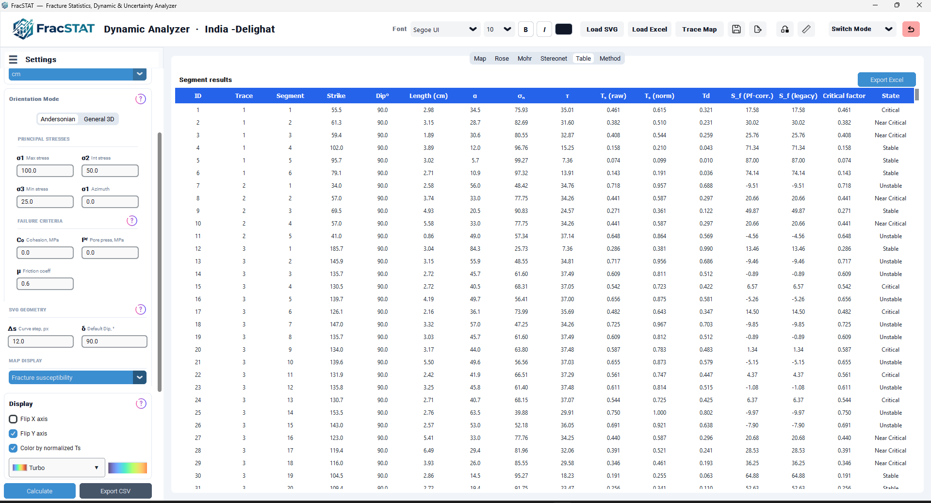
The Table Tab occupies the full main-content region of the Dynamic Analyzer window beneath the shared workspace header (font/colour controls, Load SVG/Load Excel, Save Project, Move Elements, Scale, Switch Mode, Back) and to the right of the collapsible sidebar (Profile & Units, Stress & Orientation, Display, Actions, Results summary, Selected Segment panel — all shared with the other tabs). The tab's own layout consists of three stacked regions arranged on a two-column, three-row grid:
- Row 0 — Toolbar: a transparent frame containing the section label "Segment results" (left-aligned, bold) and an "Export Excel" button (right-aligned).
- Row 2 — Data grid: a
ttk.Treeviewwidget (columns-only view, i.e. no expandable tree hierarchy) occupying column 0, paired with a verticalttk.Scrollbarin column 1. - (Row 1 is intentionally left empty as spacing in the underlying grid definition.)
The Treeview is configured with row weight 1 on grid row 2 and column weight 1 on grid column 0, so the table area expands to fill all available vertical and horizontal space as the window is resized; only the scrollbar column remains fixed-width.
3. Data Input and Underlying Data Model
The Table Tab performs no calculation of its own. It is a pure presentation layer over
self.results, the DataFrame assembled by
calculator.run_calculation() every time SlipTendencyApp.calculate()
executes (triggered by pressing "Calculate", pressing Enter in a sidebar field, loading a new
SVG or Excel/CSV file, changing the profile scale, or applying a dip-override file). The
DataFrame's construction pathway differs depending on the data source:
- SVG source — segments are read by
svg_loader.read_svg_segments(), converted from SVG pixel coordinates to physical (metre-equivalent) coordinates using the profile width/length calibration, and their strike is derived from segment geometry viamodels.segment_strike()and north-corrected viamodels.north_corrected_strike(). - Excel/CSV source — segments are read by
excel_loader.read_excel_segments(), which auto-detects one of five input schemas (raw XY segment coordinates, legacy Strike/Dip fracture planes, Trend/Plunge pole data, focal-mechanism nodal-plane tables, or FracSTAT's own exported results format) and populates the Segment dataclass's_preset_strike/_preset_dipfields directly, bypassing pixel geometry entirely.
Regardless of source, every row passed through calculator.run_calculation() is
resolved against the current principal-stress tensor (σ1, σ2, σ3), its orientation mode
(Andersonian or fully general 3-D), and the Mohr–Coulomb failure parameters (cohesion C₀, pore
pressure Pf, friction coefficient μ) that are set in the sidebar's Stress and Orientation card.
The resulting DataFrame therefore couples pure geometry (position, strike, dip, length) with the
outcome of a specific stress-field hypothesis; re-running Calculate with different stress inputs
regenerates self.results and the Table Tab automatically reflects the new numbers
on its next refresh.
3.1 Column Provenance Table
| DataFrame Field | Origin | Present For |
|---|---|---|
| ID | Sequential row index assigned in calculator.run_calculation() | All sources |
| Trace / Segment | Segment.trace_id / Segment.segment_id | All sources |
| StrikeDeg | models.segment_strike() + models.north_corrected_strike() (SVG) or Segment._preset_strike (Excel) | All sources |
| DipDeg | Sidebar "Default Dip" or per-row dip-override file (SVG) / Segment._preset_dip (Excel) | All sources |
| Length / Length_m | Physical segment length after profile-scale conversion, or Segment._preset_length for legacy Excel rows | All sources (0 for orientation-only Excel formats) |
| AlphaDeg, SigmaN, Tau | stress_on_plane_3d() / stress_on_plane_3d_general() in models.py | All sources |
| SlipTendency, SlipTendencyNorm | calculator.py; normalised by the closed-form theoretical maximum | All sources |
| DilationTendency | calculator.py | All sources |
| FractureSusceptibility, FractureSusceptibilityLegacy | calculator.py, two historical MATLAB formula variants | All sources |
| CriticalStress, CriticalStressValue, CriticalFactor, CriticalState | calculator.py Coulomb comparison (critical_factor_and_state() for the latter two) | All sources |
4. Settings and Controls
The Table Tab exposes a deliberately minimal control surface: unlike the Map, Rose, Mohr, and Stereonet tabs — each of which carries an extensive colour/geometry/typography settings panel — the Table Tab has no cosmetic settings of its own. Its only interactive controls are the Export Excel button, the column headers (for visual reference; the Treeview widget used here does not implement interactive column sorting), row selection via mouse click, and the vertical scrollbar. This design choice keeps the tab focused on its role as a neutral, complete numerical record rather than a further stylable visualisation.
4.1 Toolbar Controls
| Control | Type | Behaviour |
|---|---|---|
| "Segment results" | Static label (bold, 13 pt) | Section heading; no interactivity. |
| Export Excel | CTkButton, 120×30 px | Invokes SlipTendencyApp.export_excel(), which writes self.results to a user-chosen .xlsx workbook (sheet "Segment results") via a native Save dialog. If self.results is empty, an error dialog ("Nothing to export — Run a calculation first.") is shown instead. On success, the status bar and a confirmation dialog report the saved row count and file path. |
4.2 Data Grid Controls
| Control | Type | Behaviour |
|---|---|---|
| Column headers (×16) | ttk.Treeview "heading" cells | Display the fixed column captions (see Section 5). The "Length" heading is dynamically rewritten on every refresh to embed the active display unit, e.g. "Length (m)", "Length (cm)". |
| Row selection | ttk.Treeview single-row click / arrow-key navigation | Selecting a row fires the <<TreeviewSelect>> virtual event, handled by on_table_select(), which drives cross-tab highlighting (Section 8). |
| Vertical scrollbar | ttk.Scrollbar, orient="vertical" | Bound bidirectionally to the Treeview's yview; scrolls through all loaded rows (subject to the 1000-row rendering cap, Section 10). |
5. Column Reference and Symbol Table
Sixteen fixed columns are defined at build time and never added to or removed from at runtime; only their contents are refreshed. Each column has a physical width of 90 px and centre-anchored text. The table below gives the internal DataFrame field, the on-screen heading (including any Unicode mathematical symbol used), the physical unit or dimensionless status, the numeric formatting applied, and a one-line description of geomechanical meaning.
The Unicode symbols α, σₙ, τ, and the subscripted Tₛ are rendered directly as heading text (the
mixin imports no external font glyphs for this purpose beyond the system font already in use);
this mirrors the same symbol set defined centrally in constants.py
(SIGMA_N, TAU, T_S, T_D, S_F,
C_0, P_F) and used consistently across the Mohr, Stereonet, and
sidebar Failure-Criteria controls, so that a value bearing the same symbol always means the same
physical quantity throughout the application.
| # | Column key | Heading shown | Format | Unit | Meaning |
|---|---|---|---|---|---|
| 1 | ID | ID | integer | — | Sequential row identifier assigned during calculation; used as the Treeview row iid and as the cross-tab selection key. |
| 2 | Trace | Trace | integer | — | Parent trace/fracture-plane group identifier (multiple segments can share one trace for SVG-derived polylines). |
| 3 | Segment | Segment | integer | — | Index of this segment within its parent trace. |
| 4 | Strike | Strike | 0.0 (1 dp) | degrees | North-referenced strike azimuth of the fracture plane, StrikeDeg. |
| 5 | Dip | Dip° | 0.0 (1 dp) | degrees | Dip angle of the fracture plane, DipDeg (0–90°). |
| 6 | Length | Length (unit) | 0.00 (2 dp) | active display unit | Physical segment length; heading unit updates live with the sidebar's unit selector. |
| 7 | Alpha | α | 0.0 (1 dp) | degrees | Angle between the fracture-plane normal and the σ1 direction, AlphaDeg — governs how strongly the plane is loaded by the maximum principal stress. |
| 8 | SigmaN | σₙ | 0.00 (2 dp) | MPa | Total resolved normal stress on the plane, SigmaN. |
| 9 | Tau | τ | 0.00 (2 dp) | MPa | Resolved shear stress on the plane, Tau. |
| 10 | Ts | Tₛ (raw) | 0.000 (3 dp) | dimensionless | Raw (non-normalised) slip tendency τ/σₙ for this specific plane. |
| 11 | TsNorm | Tₛ (norm) | 0.000 (3 dp) or "—" | dimensionless, 0–1 | Slip tendency normalised by the theoretical maximum over all possible orientations for the current stress tensor; shown as an em-dash if the column is absent from self.results. |
| 12 | Td | Td | 0.000 (3 dp) | dimensionless, 0–1 | Dilation tendency, DilationTendency. |
| 13 | Sf | S_f (Pf-corr.) | 0.00 (2 dp) | MPa | Fracture susceptibility including pore-pressure and cohesion correction, FractureSusceptibility. |
| 14 | SfLegacy | S_f (legacy) | 0.00 (2 dp) or "—" | MPa | Original (pre-correction) MATLAB-formula fracture susceptibility, FractureSusceptibilityLegacy; shown as an em-dash if absent. |
| 15 | Factor | Critical factor | 0.000 (3 dp) | dimensionless | The friction coefficient required to resist the resolved shear stress, max(τ − C₀, 0) / (σₙ − Pf), CriticalFactor. Compare against the sidebar's entered friction coefficient μ to gauge how close a plane is to failure; see Section 6.6 for the zero/negative effective-stress cases. |
| 16 | State | State | text | — | The four-tier critical-fracture classification, CriticalState: "Stable" (Factor/μ < 50%), "Near Critical" (50–75%), "Critical" (75–100%), or "Unstable" (>100%); see Section 6.6. |
columns = ("ID", "Trace", "Segment", "Strike", "Dip", "Length",
           "Alpha", "SigmaN", "Tau", "Ts", "TsNorm", "Td", "Sf",
           "SfLegacy", "Factor", "State")
self.table = ttk.Treeview(tab, columns=columns, show="headings")
headings = {
    "ID": "ID", "Trace": "Trace", "Segment": "Segment",
    "Strike": "Strike", "Dip": "Dip°", "Length": "Length",
    "Alpha": "α", "SigmaN": "σₙ", "Tau": "τ",
    "Ts": "Tₛ (raw)", "TsNorm": "Tₛ (norm)",
    "Td": "Td",
    "Sf": "S_f (Pf-corr.)", "SfLegacy": "S_f (legacy)",
    "Factor": "Critical factor", "State": "State",
}
for col in columns:
    self.table.heading(col, text=headings[col])
    self.table.column(col, width=90, anchor="center")
Column and heading construction excerpted from _build_table_tab(), showing the fixed sixteen-column definition and the fixed-width, centre-anchored layout applied to every column.
6. Mathematical Background
Although the Table Tab performs no arithmetic itself, correct interpretation of its columns
requires the exact formulas used upstream in calculator.py and
models.py. This section reproduces those formulas with variable definitions so
that the table's numbers can be manually verified or compared against independent reference
calculations (e.g. legacy MATLAB slip-tendency scripts).
6.1 Symbol Definitions
| Symbol | Description | Units |
|---|---|---|
| σ1, σ2, σ3 | Maximum, intermediate, and minimum principal stress magnitudes (σ1 ≥ σ2 ≥ σ3) | MPa |
| azimuth / σ1 trend | Compass bearing of σ1 (Andersonian mode) or of the general 3-D σ1 axis | degrees from North |
| strike, dip | North-referenced strike and dip of the fracture plane | degrees |
| α | Angle between the plane's pole (normal) and the resolved σ1 axis component | degrees |
| σₙ | Normal stress resolved onto the plane | MPa |
| τ | Shear stress resolved onto the plane (magnitude of the in-plane traction component) | MPa |
| C₀ | Cohesion, the rock's inherent shear strength at zero effective normal stress | MPa |
| Pf | Pore fluid pressure acting within the fracture | MPa |
| μ | Coefficient of friction governing the Mohr–Coulomb failure envelope slope | dimensionless |
| Ts, Ts,max | Raw slip tendency and its theoretical maximum over all orientations | dimensionless |
| Td | Dilation tendency | dimensionless, 0–1 |
| Sf | Fracture susceptibility (pore-pressure corrected) | MPa |
6.2 Stress Resolution (σₙ, τ, α)
For a plane of given strike and dip, the outward unit normal is constructed from the pole
azimuth (strike + 90°) and the dip angle. In Andersonian mode (σ1 horizontal along the entered
azimuth, σ2 vertical, σ3 horizontal-perpendicular), or in the fully general 3-D mode (σ1, σ2, σ3
each independently oriented from trend/plunge inputs and combined via
principal_stress_axes_fracstat()), the normal is projected onto each principal
axis to obtain direction cosines c0, c1, c2. The resolved normal and shear stresses are then:
This is the standard Cauchy stress-resolution equation for a plane in a principal-axis coordinate frame (Jaeger et al., 2007): σₙ is the diagonal (normal) component of the traction vector and τ is the magnitude of its orthogonal in-plane component, obtained by subtracting σₙ² from the total squared traction magnitude. σₙ is floored at 1×10⁻¹² MPa in the implementation to avoid division-by-zero downstream.
6.3 Slip Tendency (Ts, TsNorm)
Slip tendency, following Morris et al. (1996), expresses how close a plane is to frictional sliding under the resolved stress state, independent of any assumed cohesion or pore pressure:
The normalised column TsNorm divides this raw value by the theoretical maximum slip tendency attainable by any plane orientation under the same stress tensor. For a diagonal (principal-axis) stress state this maximum has the closed-form solution derived from the tangent line from the origin to the outer σ1–σ3 Mohr circle:
This closed-form expression depends only on σ1 and σ3 (not on σ2, the principal-axis orientation, or which fracture planes happen to be loaded), and reproduces exactly the legacy MATLAB script's TsMax, which is computed there by a dense numerical grid-scan over all φ/θ orientation pairs. TsNorm therefore always lies in the interval [0, 1], with 1 corresponding to the single, optimally oriented plane for the given stress tensor. A superseded implementation normalised instead by the maximum Ts found only among the loaded segments; this silently disagreed with the reference value whenever the input dataset did not happen to include a near-optimal plane, and has been replaced by the closed-form calculation above.
6.4 Dilation Tendency (Td)
Dilation tendency (Ferrill and Morris, 2003) measures the propensity of a fracture to open (dilate) rather than slip, and is highest for planes whose normal is closely aligned with σ3 (minimum compressive stress), where the clamping normal stress is smallest relative to the overall stress differential.
6.5 Fracture Susceptibility (Sf, SfLegacy)
Two historically distinct MATLAB reference formulas exist for fracture susceptibility, differing by exactly the pore-pressure and cohesion terms. The Table Tab reports both simultaneously as separate columns so that either can be matched against whichever legacy script produced a comparison dataset:
Algebraically, SfLegacy = Sf + Pf whenever C₀ = 0, since the only structural difference between the two formulas is the presence of the pore-pressure subtraction and the cohesion offset inside the friction term. A lower Sf value indicates a plane closer to, or past, the failure envelope; Sf can be negative for critically or super-critically stressed planes. Read as a pore-pressure margin, the corrected form is the quantity used to set sustainable injection pressures (Streit and Hillis, 2004).
6.6 Coulomb Critical-Stress Flag (CSF)
The Mohr–Coulomb failure criterion used throughout FracSTAT is (Jaeger et al., 2007; Sibson, 1985):
This criterion is evaluated for every row during calculation and stored in the results DataFrame
as the boolean CriticalStress flag (with CriticalStressValue,
CoulombMargin and EnvelopeDistance alongside it), but it is not one of
the Table Tab's 16 visible columns: what the table surfaces is the finer-grained
Critical factor and State pair derived from the same numbers.
The flag itself is exactly the boolean condition drawn as the Coulomb failure envelope on the
Mohr tab and reflected in the map/rose colour scale when "Critical fractures" is the selected
attribute.
Critical factor is the friction coefficient the plane would need in order to resist
its resolved shear, max(τ − C₀, 0) / (σₙ − Pf), which is directly comparable with the μ ≈ 0.6–0.85
range measured for most rock types
(Byerlee, 1978), and State bands the
ratio of that demand to the entered μ at 50% / 75% / 100%. Two degenerate cases are handled
explicitly rather
than producing a division error: if the effective normal stress σₙ − Pf is zero or negative the
factor is 0 when there is no driving shear and +∞ otherwise (so a tensile plane carrying shear
reports as Unstable), and if μ itself is zero the ratio is +∞ whenever the factor is positive.
Because the driving shear is floored at zero, a plane whose resolved τ lies below its cohesion
reports a factor of exactly 0 rather than a negative value.
7. Algorithms and Internal Workflow
7.1 Tab Construction — _build_table_tab()
Executed once, during SlipTendencyApp._build_layout(), after the tab's Qt container
frame has been created by the CTkTabview. The method performs, in order:
- Grid configuration — row 2 (the data grid row) and column 0 are given weight 1 so the table stretches to fill the tab.
- Theme application —
configure_table_style()is invoked immediately so the Treeview's ttk style exists before any rows are inserted (see Section 7.3). - Toolbar construction — a transparent CTkFrame with the "Segment results" label and Export Excel button, gridded at row 0.
- Column and heading setup — the fifteen-element columns tuple is used both
to instantiate the
ttk.Treeview(columns=columns, show="headings")(note:show="headings"suppresses the default first "#0" tree column, so the widget behaves as a flat, non-hierarchical grid) and to populate each column's heading text from the headings dictionary and a fixed 90 px, centre-anchored column width. - Scrollbar wiring — a
ttk.Scrollbaris created withcommand=self.table.yviewand the Treeview'syscrollcommandis bound back to the scrollbar, establishing the standard bidirectional Tk-style scroll contract. - Event binding — the Treeview's
<<TreeviewSelect>>virtual event (fired by the Treeview whenever the widget's selection changes, whether by mouse or keyboard) is bound toon_table_select.
No rows are inserted at build time; the table remains empty until the first
refresh_table() call, which normally follows the first successful calculation.
7.2 Selection Handling — on_table_select()
This callback fires on every change to the Treeview's internal selection, including selections
made programmatically by refresh_table() itself when it restores a previously
highlighted row after a redraw. To avoid a feedback loop or redundant recomputation, the
handler follows this short-circuit sequence:
- Read
self.table.selection()— a tuple of currently selected item identifiers (iids). If empty (e.g. the user clicked empty space below the last row), the handler returns immediately. - Parse the first selected iid as an integer with
int(selection[0]). The iid was set at insertion time tostr(int(row.ID)), so this recovers the numeric segment ID. If parsing fails (defensive — should not occur given how iids are always assigned), the handler returns silently. - Compare the parsed ID against
self.selected_segment_id. If they are already equal — for example becauserefresh_table()just re-selected the same row the user had previously picked — the handler returns without further action, preventing an unnecessary cascade of redraws across the Map, Mohr, and Stereonet tabs. - Otherwise, call
self.select_segment(segment_id), the shared cross-tab selection routine defined onSlipTendencyAppitself (see Section 8).
def on_table_select(self, _event=None):
    selection = self.table.selection()
    if not selection:
        return
    try:
        segment_id = int(selection[0])
    except ValueError:
        return
    if segment_id == self.selected_segment_id:
        return
    self.select_segment(segment_id)
on_table_select() in full — the short-circuit guards prevent a redundant cascade of redraws whenever the incoming selection already matches the current cross-tab selection.
7.3 Theming — configure_table_style()
The Treeview (unlike the regular CTk* controls) does not automatically follow
FracSTAT's light/dark
colour tokens, so this method explicitly configures a ttk.Style object every time
it is called. Under the PySide6 backend, ttk.Style is the
ui_common.qtk.ttk compatibility shim: the options configured here are translated
into Qt stylesheet (QSS) rules and applied to the underlying QTreeWidget. The
theme_use("clam") call is retained for API compatibility and has no visual effect
on the Qt backend. The method then branches on
self.appearance_var.get():
| Element | Light mode | Dark mode |
|---|---|---|
| Treeview background / field background | #FFFFFF | #111821 |
| Treeview foreground (row text) | #1F2933 | #E6EDF3 |
| Row height | 26 px | 26 px |
| Border width | 0 (flat) | 0 (flat) |
| Heading background | #2563EB | #1F6AA5 |
| Heading foreground | white | white |
| Selected-row background | #DBEAFE | #255B7D |
| Selected-row foreground | #1F2933 | #FFFFFF |
configure_table_style() is called both at tab construction
and whenever SlipTendencyApp.change_appearance() runs, ensuring the Treeview's
colours stay synchronised even though FracSTAT's Dynamic Analyzer is presently fixed to a
single light theme at the application level (change_appearance() always forces
"Light"); the dark-mode branch remains implemented and reachable should the appearance toggle
be re-enabled.
7.4 Refresh Algorithm — refresh_table()
refresh_table() is the workhorse of the tab and is called every time
self.results changes (after calculate(), after
select_segment(), and after clear_selection()). Its steps are:
- Clear existing rows:
self.table.delete(*self.table.get_children())removes every currently displayed row unconditionally, regardless of how many there are. - Empty-result guard: if
self.results.empty, the method returns immediately, leaving the table blank — this is the state shown before any file has been loaded or calculated. - Dynamic unit relabelling:
self.table.heading("Length", text=f"Length ({self.unit_label()})")rewrites the Length column's heading text to reflect whatever display unit (m, cm, mm, km) is currently active in the sidebar, so the heading never becomes stale after a unit-conversion action. - Optional-column detection:
has_ts_normandhas_sf_legacyare booleans testing whether "SlipTendencyNorm" and "FractureSusceptibilityLegacy" exist as columns inself.results. Becausecalculator.run_calculation()always adds both columns in the current implementation, these guards are defensive — they protect the table from raising anAttributeErrorif it is ever driven by an older or externally supplied results DataFrame that lacks one of the derived columns, substituting the placeholder character "—" (em dash) instead. - Row insertion loop:
self.results.head(1000).itertuples(index=False)iterates at most the first 1000 rows of the results DataFrame (see Section 10 for the rationale). For each row, the displayed values are formatted (see Section 5's Format column) and inserted withself.table.insert("", "end", iid=str(int(row.ID)), values=(...)). Using the segment's own ID as the Treeview item identifier is what allowson_table_select()to recover the numeric ID directly from the widget's selection state without a separate lookup table. - Selection restoration: if
self.selected_segment_id is not Noneand its string form exists among the freshly inserted children, the method callsself.table.selection_set(selected_iid)followed byself.table.see(selected_iid). This re-applies the previously active selection (which was necessarily cleared by step 1's blanket delete) and scrolls the view so the selected row is visible, giving the appearance of a persistent highlight across recalculations even though the underlying Qt items were fully destroyed and rebuilt.
8. Cross-Tab Selection Synchronisation
The Table Tab does not maintain its own notion of "the selected segment"; it defers entirely to
SlipTendencyApp.select_segment(segment_id), the single shared routine also invoked
by mouse-picking on the Map (on_map_pick), point-picking on the Mohr diagram
(on_mohr_pick), and pole-picking on the Stereonet
(on_stereonet_pick). When a Table Tab row is clicked, the following chain
executes:
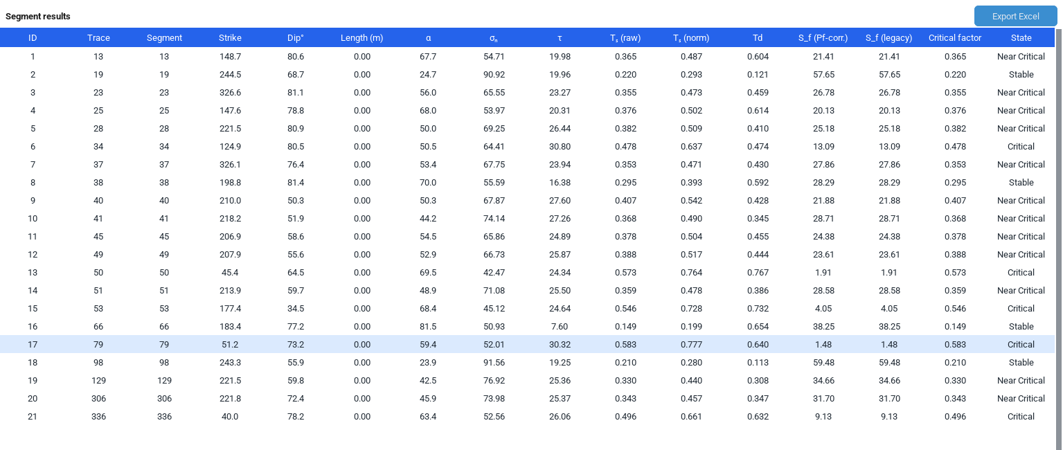
on_table_select()resolves the clicked row's ID and callsself.select_segment(segment_id).select_segment()looks up the matching row inself.results, setsself.selected_segment_id, updates the sidebar's "Selected Segment" text panel (segment_info_text()) with a full geometric/orientation/stress/tendency summary, updates the Mohr diagram's information panel and coloured status badge (Critical / Near envelope / Stable, based on CoulombMargin and a 5%-of-max-τ tolerance band), and updates the Stereonet's pole-inspector text.select_segment()then callsself.refresh_table()itself, so the Table Tab's own view re-synchronises its highlighted row even when the selection originated elsewhere (e.g. clicking a point on the Mohr diagram highlights the same segment's row in the Table Tab automatically).- Finally,
select_segment()triggers preserve-view redraws of the Map (_draw_map(preserve_view=True)), Mohr (_draw_mohr(preserve_view=True)), and Stereonet (_draw_stereonet()) so the selected segment is visually emphasised (halo/outline markers, annotation labels) everywhere simultaneously.
This design means the Table Tab is both a consumer and a producer of selection state: any tab's
picking interaction is reflected in the Table Tab's highlighted row, and clicking a Table Tab
row is reflected everywhere else. The optional switch_to_map parameter of
select_segment() (used by the Mohr and Stereonet tabs' "Show in Map" buttons) is
not exercised from the Table Tab itself, which never forces a tab switch.
Clearing the selection — via the Mohr or Stereonet tabs' "Clear Selection" buttons, which call
SlipTendencyApp.clear_selection() — sets self.selected_segment_id
back to None and calls refresh_table(), which then finds no matching
iid in step 6 of Section 7.4 and leaves the table with no row highlighted.
9. Statistical Content and Relationship to the Sidebar Summary
The Table Tab itself performs no aggregation; the workspace-level statistical summary (traces,
segments, Max Tₛ, Mean Tₛ, total length, and critical-fracture count) is computed separately in
SlipTendencyApp.refresh_summary() and displayed in the sidebar's "Results" card,
not inside the Table Tab. However, because the Table Tab exposes every underlying row value, it
is the natural tool for verifying those aggregate statistics manually: for instance, the
sidebar's "Max Tₛ" / "Mean Tₛ" tiles are computed over whichever attribute (SlipTendency,
SlipTendencyNorm, DilationTendency, FractureSusceptibility(Norm), or CriticalStressValue) is
currently selected in the "Map Display" dropdown, and the exact numeric contributors to that
maximum or mean can be located, sorted by eye, and cross-checked row-by-row in the Table Tab.
9.1 Interpreting Column Distributions
| Observation in the Table Tab | Geomechanical interpretation |
|---|---|
| Many rows with CSF = "Yes" | The current stress tensor is close to, or exceeds, the assumed failure envelope for a large fraction of the fracture population — indicative of a critically stressed fracture network with elevated potential for fluid flow along reactivated planes. |
| TsNorm clustered near 1.0 for a subset of rows | Those planes are oriented close to the theoretically optimal slip-prone orientation for the current σ1–σ3 differential; in an Andersonian regime this typically corresponds to strikes sub-parallel to σ1 with dip near the frictional-lock angle (~30° from σ1 for μ ≈ 0.6). |
| Td consistently higher than Ts for the same rows | Planes are more prone to opening-mode dilation than to frictional slip under the current stress state — relevant when assessing which fractures are more likely to act as open conduits versus shear-reactivated conduits. |
| Sf and SfLegacy diverging substantially | Indicates a non-trivial pore-pressure (Pf) or cohesion (C₀) input; the magnitude of the divergence is, by construction, approximately equal to Pf when C₀ = 0 (Section 6.5). |
10. Performance Optimisation
The Table Tab includes two deliberate performance safeguards, both aimed at keeping the Qt main
loop responsive when self.results contains a very large number of segments (dense
SVG trace networks with fine curve-tessellation settings can readily produce several thousand
to tens of thousands of rows):
- Row cap —
refresh_table()iterates onlyself.results.head(1000), i.e. at most the first one thousand rows in DataFrame order, regardless of the true row count.ttk.Treeviewinserts are individually expensive Qt operations, and inserting tens of thousands of rows synchronously on the main GUI thread would visibly freeze the interface for a period proportional to row count. Capping at 1000 keeps the insertion loop's wall-clock cost small and bounded irrespective of dataset size. This cap affects only the Table Tab's on-screen display and selection restoration; it has no effect on the Map, Rose, Mohr, Stereonet, or Excel-export pathways, all of which continue to operate on the full, uncappedself.resultsDataFrame. - Full-clear-and-rebuild rather than incremental diffing — every refresh deletes all existing rows before reinserting, rather than attempting to compute a minimal diff against the previous state. This trades a theoretically larger amount of Qt work per refresh for substantially simpler, more robust code with no risk of stale rows, orphaned iids, or column-value drift; given the 1000-row cap, the practical cost of full deletion-and-reinsertion is small.
No caching layer, background thread, or asynchronous loading is used for the Table Tab specifically (contrast with, for example, the Static Analyzer's asynchronous SVG/Excel loaders or the Connectivity tab's lazy, tab-click-triggered recomputation) — the table's own render cost is low enough, given the row cap, that synchronous execution on the main thread does not perceptibly delay the interface.
10.1 Practical Implication of the 1000-Row Cap
When a dataset exceeds 1000 segments, the on-screen table displays only the first 1000 in DataFrame order (which is the order segments were produced during loading/calculation — typically grouped by trace for SVG sources, or by input-file row order for Excel/CSV sources). Analysts working with very dense networks should rely on the Export Excel action to obtain the complete, uncapped dataset for full-population statistical analysis, and should not assume the visible table represents the entire fracture population once the row count exceeds one thousand.
11. Export Functionality
The Export Excel button is the Table Tab's only outward data-transfer control; it delegates to
SlipTendencyApp.export_excel(), a method shared at the workspace level (the Table
Tab does not implement its own export logic). The behaviour is:
- Guard: if
self.results.empty, an error dialog ("Nothing to export" / "Run a calculation first.") is shown and the method returns without opening a file dialog. - Default directory resolution: the method attempts to read a configured
default export path from the application's persisted settings
(
pages.settings_page.load_app_settings()); if unavailable or invalid, no initial directory is pre-selected and the OS default is used. - Save dialog: a native "Save As" dialog is presented with a .xlsx default extension and an "Excel workbook" file-type filter.
- Write:
self.results.to_excel(filename, index=False, sheet_name="Segment results")writes the complete (uncapped) DataFrame — every row and every column, including any columns not rendered in the on-screen table — to a single-sheet workbook. This means the exported file is a strict superset of what is visually displayed, and is the recommended path for any downstream analysis requiring the full dataset. - Confirmation: the workspace status bar is updated with the number of exported rows and file path, and a confirmation dialog displays the saved path.
export_csv(), triggered from the
sidebar's "Export CSV" action button rather than from within the Table Tab) is available at
the workspace level using the same underlying self.results DataFrame and the same
empty-result guard, for workflows that prefer a plain-text tabular format over a native Excel
workbook.
12. Practical Examples
12.1 Example 1 — Verifying a Slip-Tendency Calculation by Hand
An analyst loads an SVG fracture-trace map, sets σ1 = 104.7 MPa, σ2 = 60.3 MPa, σ3 = 47.1 MPa in Andersonian mode with azimuth 0°, and presses Calculate. To manually verify the reported Tₛ (norm) value for segment ID 12, the analyst locates row ID = 12 in the Table Tab (using the scrollbar or, for large datasets, exporting to Excel and using a spreadsheet find function), reads off StrikeDeg, DipDeg, σₙ, and τ, and reproduces α, σₙ, τ using the equations of Section 6.2, then Ts and TsNorm using Section 6.3's formulas — including the closed-form Ts,max — confirming the value shown in the Tₛ (norm) column.
12.2 Example 2 — Cross-Referencing a Critical Segment Between Table and Mohr Diagram
After calculation, the analyst scans the CSF column in the Table Tab for rows marked "Yes", identifying the subset of the fracture population predicted to be critically stressed under the current stress hypothesis. Clicking one such row (say ID = 47) immediately re-draws the Mohr tab with segment 47's point highlighted with a bold outline and "ID 47" annotation sitting on or beyond the shaded failure envelope, and simultaneously highlights the same segment on the Map and Stereonet tabs — allowing the analyst to confirm both the stress-space position (Mohr) and the real-world geometric position and orientation (Map/Stereonet) of that specific fracture in one interactive step.
12.3 Example 3 — Comparing Legacy and Corrected Fracture Susceptibility
When importing results intended to reproduce an older MATLAB workflow that used the original Sf = σₙ − τ/μ formula (no pore-pressure correction), the analyst compares the Sf (Pf-corr.) and Sf (legacy) columns directly in the Table Tab. If the two differ by a near-constant offset across all rows and the sidebar's Pore press. (MPa) field is non-zero, this offset is expected and equals approximately Pf (Section 6.5); a non-constant offset instead flags a non-zero cohesion input interacting with the two formulas differently and should prompt the analyst to check the Failure Criteria card's Cohesion (MPa) field.
12.4 Example 4 — Exporting Full Results for a Technical Report
For inclusion of a complete segment-level results appendix in a technical report, the analyst
clicks Export Excel, saves the workbook, and opens it in Excel or an equivalent spreadsheet
application; every row of self.results — not merely the 1000 rows visible in the
on-screen table for a large network — is present, including columns (such as raw pixel
coordinates, RawX1/RawY1/RawX2/RawY2, or focal-mechanism metadata for geographic datasets) that
are not shown in the Table Tab's fifteen-column view at all.
13. Geological and Geomechanical Interpretation
The Table Tab's numerical content supports several standard structural-geology and reservoir-geomechanics interpretation workflows built on the Wallace–Bott hypothesis (that slip on a pre-existing fracture occurs in the direction of maximum resolved shear traction (Wallace, 1951; Bott, 1959)) and its slip/dilation-tendency derivatives:
- Fault/fracture reactivation risk assessment — rows with high TsNorm and CSF = "Yes" identify the subset of a mapped fracture network most susceptible to shear reactivation under the assumed in-situ or induced stress state, directly informing induced-seismicity risk screening around injection or production operations.
- Fluid-flow pathway prediction — high-Td fractures are preferentially interpreted as open, dilated conduits, whereas high-Ts, low-Td fractures are better candidates for shear-enhanced (but not necessarily dilated) permeability; comparing the Td and Ts (norm) columns row-by-row across a population supports discriminating between these two permeability-enhancement mechanisms.
- Wellbore-stability and completion design — the Sf column's sign and magnitude for fractures intersecting a planned or existing wellbore trajectory is a standard input into whether a given natural fracture is likely to be a fluid-loss zone or a slip hazard during drilling or stimulation.
- Stress-tensor sensitivity testing — because every column updates immediately after a recalculation, an analyst can iterate the σ1/σ2/σ3 magnitudes or orientation inputs and observe, row-by-row in the Table Tab, how sensitive the critically-stressed subset (CSF) and the slip/dilation-tendency rankings are to the assumed stress state — a standard uncertainty-bracketing exercise given that in-situ stress magnitudes and orientations are rarely known with high precision (Zoback, 2007).
14. Implementation Notes
- Mixin architecture —
TableTabis a bare Python mixin class (it does not inherit fromctk.CTkFrameor any Qt widget); its methods assume the presence ofself.tabs,self.results,self.selected_segment_id,self.appearance_var,self.unit_label(), andself.select_segment(), all of which are supplied bySlipTendencyAppat composition time via Python's standard multiple-inheritance MRO (SlipTendencyApp(WorkspaceHeaderMixin, MapTab, RoseTab, MohrTab, TableTab, MethodTab, StereonetTab, ctk.CTkFrame)). - Widget technology — the Table Tab is the only tab in the Dynamic Analyzer
that uses the
ui_common.qtk.ttk.Treeview/Scrollbarwidgets rather than the regularCTk*controls (there is no built-in multi-column tabularCTk*widget); the Treeview is aQTreeWidgetsubclass, which is why it requires its own explicitttk.Styletheming rather than relying on the automatic light/dark colour tuples the other qtk widgets accept. - Item identifiers (iids) — using
str(int(row.ID))as the Treeview iid, rather than an auto-generated internal iid, is what allows O(1) mapping between a clicked row and its underlying segment ID, and what allows selection restoration (Section 7.4, step 6) to work by simple string containment testing ("in self.table.get_children()") without maintaining a separate lookup dictionary. - Row-value construction is done with pandas'
itertuples(index=False)(McKinney, 2010), which is significantly faster thaniterrows()for this row count and, unlikeiterrows(), preserves each column's native dtype as an attribute (row.ID,row.StrikeDeg, etc.) rather than boxing every value into a single mixed-type Series per row. - No sorting state is persisted or implemented — clicking a column heading
does not resort the Treeview in the current implementation; the table always reflects
self.results' native row order (segment ID order). - Thread safety —
refresh_table()andon_table_select()are both expected to run exclusively on the Qt main thread, consistent with the rest of the Dynamic Analyzer; no locking or thread-marshalling is implemented because no other thread ever mutatesself.resultsorself.selected_segment_idconcurrently with the Table Tab's own execution.
15. References
Sources are listed alphabetically within each group. In-text citations throughout this page link to the corresponding entry below.
15.1 Stress Resolution and Failure Criteria
- Byerlee, J. (1978). Friction of rocks. Pure and Applied Geophysics, 116(4–5), 615–626. https://doi.org/10.1007/BF00876528
- Jaeger, J. C., Cook, N. G. W., & Zimmerman, R. W. (2007). Fundamentals of Rock Mechanics (4th ed.). Blackwell Publishing, Oxford. ISBN 978-0-632-05759-7. (Mohr–Coulomb failure criterion and stress-transformation equations.)
- Sibson, R. H. (1985). A note on fault reactivation. Journal of Structural Geology, 7(6), 751–754. https://doi.org/10.1016/0191-8141(85)90150-6
- Zoback, M. D. (2007). Reservoir Geomechanics. Cambridge University Press. https://doi.org/10.1017/CBO9780511586477
15.2 Tendency and Susceptibility Metrics
- Bott, M. H. P. (1959). The mechanics of oblique slip faulting. Geological Magazine, 96(2), 109–117. https://doi.org/10.1017/S0016756800059987
- Ferrill, D. A., & Morris, A. P. (2003). Dilational normal faults. Journal of Structural Geology, 25(2), 183–196. https://doi.org/10.1016/S0191-8141(02)00029-9
- Morris, A., Ferrill, D. A., & Henderson, D. B. (1996). Slip-tendency analysis and fault reactivation. Geology, 24(3), 275–278. https://doi.org/10.1130/0091-7613(1996)024<0275:STAAFR>2.3.CO;2
- Streit, J. E., & Hillis, R. R. (2004). Estimating fault stability and sustainable fluid pressures for underground storage of CO₂ in porous rock. Energy, 29(9–10), 1445–1456. https://doi.org/10.1016/j.energy.2004.03.078
- Wallace, R. E. (1951). Geometry of shearing stress and relation to faulting. The Journal of Geology, 59(2), 118–130. https://doi.org/10.1086/625831
15.3 Software
- Harris, C. R., Millman, K. J., van der Walt, S. J., Gommers, R., Virtanen, P., Cournapeau, D., … Oliphant, T. E. (2020). Array programming with NumPy. Nature, 585(7825), 357–362. https://doi.org/10.1038/s41586-020-2649-2
- McKinney, W. (2010). Data structures for statistical computing in Python. In Proceedings of the 9th Python in Science Conference (pp. 56–61). https://doi.org/10.25080/Majora-92bf1922-00a
Methods statement for the Table Tab. If a table produced or exported by this tab appears in a publication, the details below are what a reader needs in order to reproduce it, and are what the citations above assume:
Per-fracture resolved normal and shear stress computed by Cauchy transformation in the principal-axis frame (Jaeger et al., 2007) for σ1/σ2/σ3 = … MPa, P_f = … MPa, C₀ = … MPa and μ = …, with principal axes built in Andersonian or general 3-D mode as stated. Reported metrics are slip tendency and its closed-form normalisation (Morris et al., 1996), dilation tendency (Ferrill and Morris, 2003), and fracture susceptibility in both the pore-pressure- and cohesion-corrected form (Streit and Hillis, 2004) and the uncorrected legacy form (Section 6.5). Computed with pandas (McKinney, 2010) over NumPy (Harris et al., 2020). Report the full stress tensor, the orientation mode, and which susceptibility column is quoted; note that the on-screen grid is capped at 1000 rows whereas the export contains every row (Section 10.1).