Uncertainty Monte Carlo Tab

Implemented in uncertainty_montecarlo_tab.py and rendered through the shared uncertainty_sampling_tab.py workspace builder, the Monte Carlo Simulation tab is the primary probabilistic fault-stability analysis environment within the FracSTAT Uncertainty Analyzer. It lets a structural geologist, geomechanical engineer, or reservoir engineer propagate measurement and interpretation uncertainty in stress magnitudes, rock-strength parameters, pore pressure, and fault orientation through a deterministic Mohr–Coulomb fault-stability calculation, producing a fully probabilistic characterization of slip tendency, dilation tendency, fracture susceptibility, and Coulomb failure potential for one or many faults simultaneously.

Unlike a conventional deterministic geomechanical assessment — which assigns a single value to each input parameter and returns a single stability verdict — the Monte Carlo tab treats every geomechanical input as a random variable governed by a user-selected probability distribution. Thousands of independent realizations of the fault–stress system are drawn, each realization is passed through the same physical stability equations used elsewhere in FracSTAT, and the resulting population of outcomes is summarized statistically — yielding defensible, quantifiable answers to questions such as "what is the probability that this fault will fail under current reservoir conditions?" rather than a single pass/fail label that hides the underlying uncertainty.

Because uncertainty_montecarlo_tab.py itself is a thin dispatcher — it sets sampling_method="mc" and immediately delegates construction of the entire tabbed workspace to UncertaintySamplingTab.build() — this guide documents the complete Monte Carlo workflow as experienced by the user, including the six analysis sub-modules that appear as nested tabs beneath "Monte Carlo Simulation": Geomechanics, Statistics, Sensitivity, Visualization, Spatial Probability Map, and Validation & Export. Each of these sub-modules operates on the same underlying Monte Carlo realization set and is therefore an integral part of the Monte Carlo analysis, even though its implementation is factored into separate source files for maintainability.

1. Purpose and Scope

1.1 Intended Audience

• Structural geologists and geomechanical analysts performing fault-reactivation and induced-seismicity risk screening.
• Reservoir engineers evaluating injection- or depletion-induced pore-pressure changes on pre-existing faults.
• Geohazard and CO₂-storage risk assessors requiring probabilistic, auditable slip- and dilation-tendency estimates.
• Software QA engineers and technical reviewers validating the scientific correctness of FracSTAT outputs.

1.2 Document Conventions

Throughout this guide, variable names shown in the mathematical background sections correspond directly to the internal computational quantities used by the module (e.g. σ1, σ2, σ3 for the major, intermediate, and minor principal stresses). GUI labels are reproduced exactly as they appear on screen and are set in bold. Equation numbers are provided for cross-referencing between the Mathematical Background (Section 6) and the Algorithms (Section 7).

2. Position within the FracSTAT Architecture

The Uncertainty Analyzer is one of three principal analysis workspaces in FracSTAT, alongside the Static Analyzer and the Dynamic Analyzer. Unlike those two workspaces, which operate on deterministic fracture-trace geometry digitized from an image or SVG, the Uncertainty Analyzer is intentionally decoupled from image-based tracing: its input is a tabular Excel/CSV data set describing one or more fault planes and their associated geomechanical properties. The workspace header therefore disables the "Load SVG", "Scale", and "Trace Map" controls and enables only "Load Excel", reflecting this different, tabular data model.

The Monte Carlo tab and its sibling, the Latin Hypercube Sampling (LHS) tab, are the two sampling-method entry points into an otherwise identical analysis pipeline. Both are thin wrappers around the shared UncertaintySamplingTab.build() routine, differing only in the string passed for sampling_method ("mc" or "lhs"), which is later resolved by the sampling engine into a specific pseudo-random-number generation strategy (see Section 7.1). Every other element of the workspace — the input-loading logic in uncertainty_app.py, the fault-preparation and column-alias resolution in sampling_engine.py, the physical stability equations in uncertainty_calculator.py, and the six analysis sub-tabs — is shared code, so a Monte Carlo run and an LHS run for the same input data and settings are directly comparable and, at sufficiently large sample sizes, should converge to the same statistical answer.

2.1 Relationship to Other FracSTAT Modules

Module	Relationship to Monte Carlo Tab
uncertainty_app.py	Hosts the workspace shell, header controls, Excel/CSV loading pipeline, autosave, and font/typography propagation used by the Monte Carlo tab.
uncertainty_sampling_tab.py	Builds the shared tab layout (Geomechanics, Statistics, Sensitivity, Visualization, Spatial Probability Map, Validation & Export) and orchestrates the run/cancel/threading logic invoked when the user clicks Run Monte Carlo Simulation.
sampling_engine.py	Implements generate_samples(), the core routine that draws Monte Carlo variates and evaluates fault stability for every realization and every selected fault.
distributions.py	Provides the probability-distribution registry (Normal, Truncated Normal, Lognormal, Gamma, Beta, Uniform) used to transform unit-uniform coordinates into physical parameter values.
uncertainty_calculator.py	Implements the deterministic Mohr–Coulomb fault-stability physics (calculate_fault_stability) applied identically to every Monte Carlo realization.
validation.py / validation_module.py	Provide convergence diagnostics, analytical benchmark checks, reproducibility metadata, and CSV/Excel export of the Monte Carlo result set.
Static/Dynamic Analyzer	Independent workspaces; the Uncertainty Analyzer deliberately does not share its loaded input file or results with them (see _ws_on_switch in uncertainty_app.py).

3. Interface Overview

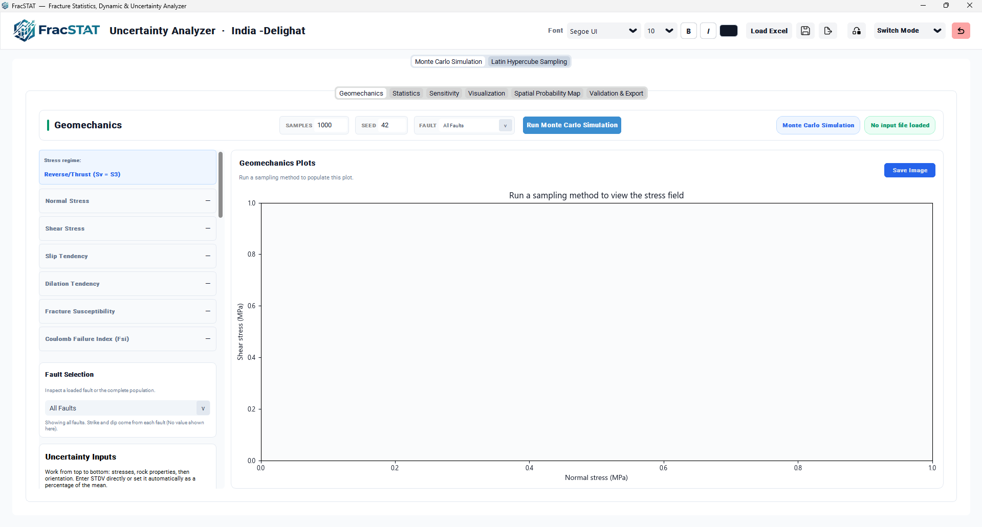
Selecting the Monte Carlo Simulation tab presents a two-level tabbed interface. The outer level (Monte Carlo Simulation vs. Latin Hypercube Sampling) selects the sampling method; the inner level presents the six analysis sub-modules described below. All six sub-modules read from the same shared context dictionary (the context object created once per outer tab in UncertaintySamplingTab.build), so a single simulation run populates every sub-module simultaneously, and only the currently visible sub-module's plot is redrawn at any moment for responsiveness (see Section 12.2).

3.1 Shared Controls Bar

Every one of the six sub-tabs presents an identical, persistent controls bar at its top, giving the user access to the shared simulation parameters regardless of which analysis view is currently active:

Control	Type	Function
SAMPLES	Numeric entry	Number of Monte Carlo realizations to draw per fault (default 1000; validated to the range 10–100,000).
SEED	Numeric entry	Integer seed for the pseudo-random number generator, guaranteeing bit-for-bit reproducible realizations (default 42).
FAULT	Scrollable dropdown	Selects "All Faults" (population-level analysis) or an individual loaded fault by ID for a single-fault deep dive.
Run Monte Carlo Simulation	Button	Validates all inputs, launches the sampling worker thread, and displays the full-screen progress overlay.
Sampling-method badge	Static label	Displays "Monte Carlo Simulation" to confirm which sampler produced the currently displayed results.
Input-source badge	Static label bound to loaded_source_var	Displays the file name (and worksheet, if applicable) of the currently loaded fault data set.
Cancel (floating)	Button, appears only during a run	Signals the background worker thread to stop at its next safe checkpoint via a threading.Event.

3.2 The Six Analysis Sub-Tabs

Sub-tab	Primary Purpose
Geomechanics	Defines every probabilistic input (stresses, strength, pore pressure, orientation), the stress regime, and displays Mohr-circle/scatter diagrams of the sampled stress state.
Statistics	Descriptive statistics (mean, SD, median, mode, percentiles, confidence interval) and histogram / input-response plots for any single metric or input.
Sensitivity	Global sensitivity analysis (Standardized Regression Coefficients and Partial Rank Correlation Coefficients) presented as a tornado diagram.
Visualization	A publication-oriented plotting library with single-plot, four-panel dashboard, and five predefined multi-panel scientific layouts.
Spatial Probability Map	Projects per-fault probability-of-failure and uncertainty-width metrics onto real-world fault coordinates loaded from a separate coordinate file.
Validation & Export	Displays convergence, analytical-benchmark, and reference-solution validation status, previews the full realization table, and exports results to CSV or Excel.

Figure 3.1 — Monte Carlo workspace layout: annotated screenshot showing the shared controls bar, the six analysis sub-tab headers, and the Geomechanics sidebar/plot split layout.

4. Data Input and Preprocessing

The Monte Carlo tab consumes tabular fault data loaded through the workspace header's Load Excel control, handled by _load_excel_file / _read_uncertainty_input_file in uncertainty_app.py. Loading occurs on a background thread so the Qt event loop remains responsive, with a full-screen loading overlay shown while the file is parsed.

4.1 Supported File Types

• .csv — read directly with pandas.read_csv.
• .xlsx / .xls — opened with pandas.ExcelFile; if the workbook contains more than one worksheet, a modal Select Worksheet dialog is presented (single-sheet workbooks load automatically with no prompt).

4.2 Column Alias Resolution

Column names in real-world spreadsheets are inconsistent ("Sigma 1" vs. "Sigma1" vs. "σ_1"). The module normalizes every header by lower-casing it, replacing non-alphanumeric characters with spaces, and collapsing repeated whitespace (_normalise_name), then matches the normalized header against a registry of accepted aliases (_COLUMN_ALIASES) for each logical field. This makes column matching case-insensitive and tolerant of spacing/punctuation differences.

Logical Field	Accepted Header Aliases (case/spacing-insensitive)
fault_id	ID No, ID, Frac_ID, Fault_ID, Fracture_ID, Fault Name, Fault_Name
strike	Strike
dip	Dip
sigma1 / sigma2 / sigma3	Sigma 1 / Sigma 2 / Sigma 3 (and underscore variants)
friction	Friction Coefficient, Friction, mu
cohesion	Cohesion, C0, C, Cohesive Strength
pore_pressure	Pore Pressure, Pore_Pressure, Pf
shmax	SH max, SHmax, S Haz, Shaz, Maximum Horizontal Stress Azimuth

4.3 Validation Rules Applied at Load Time (prepare_faults)

• Strike and Dip columns are mandatory; their absence raises an explicit error identifying which column is missing.
• Strike and Dip are coerced to numeric with pandas.to_numeric(errors="coerce"); any resulting NaN triggers a validation failure listing that Strike/Dip must be finite for every row.
• Strike must satisfy 0 ≤ Strike < 360°; Dip must satisfy 0° ≤ Dip ≤ 90°.
• If a Fault ID column is present, IDs are cast to string, whitespace-trimmed, and checked for blank or duplicate values; either condition raises an error before any sampling can begin.
• If a Fault ID column is absent, sequential integer identifiers (1, 2, 3, …) are assigned automatically.
• Optional columns (sigma1, sigma2, sigma3, friction, cohesion, pore_pressure, shmax) are coerced numeric where present; when absent for a given fault, the corresponding sidebar mean value in the Geomechanics tab is used instead.

4.4 Fault Selector and the All Faults / Single-Fault Duality

Every sub-tab shares one fault_selection_var. Selecting All Faults samples every loaded fault at the configured sample size and concatenates the results into one realization table tagged by fault_id; selecting an individual fault restricts the Strike/Dip/stress means to that fault's row and (if orientation fields are otherwise blank) draws the given number of realizations for that fault alone. To avoid redundant computation, an All Faults run is also cached per individual fault: selecting a single fault after an All Faults run instantly slices the cached population for that fault_id rather than re-running the sampler (see Section 12.1).

5. Settings and Controls

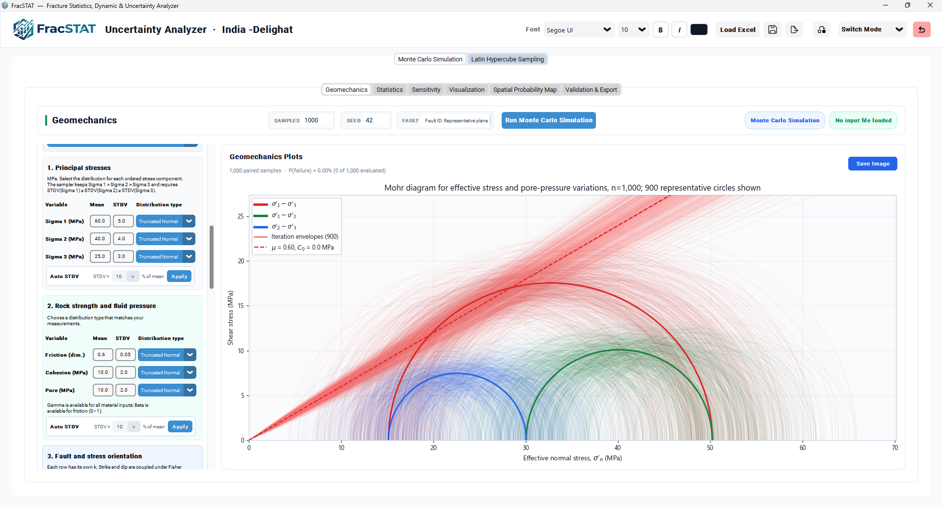
The Geomechanics sub-tab is where every stochastic input to the Monte Carlo simulation is configured. Its sidebar is organized into four numbered cards presented top-to-bottom in the recommended workflow order: stress regime, principal stresses, rock strength/fluid pressure, and fault/stress orientation, followed by the effective-stress toggle.

5.1 Stress Regime Selector

A single dropdown selects which principal stress is assumed vertical (S_v), following the Andersonian classification of faulting regimes. This selection does not alter the sampled σ1 > σ2 > σ3 ordering used for display and statistics; it only controls how those three sampled stresses are remapped onto the fault-normal stress calculation performed by calculate_fault_stability (see Section 6.4 and Section 7.4).

UI Label	Regime	Vertical Stress Assignment
Normal Faulting (Sv = S1)	normal	σ1 (largest) is vertical; internally remapped so Sv occupies the σ3 slot fed to the stability calculator.
Strike-Slip (Sv = S2)	strike_slip	σ2 (intermediate) is vertical; remapped into the σ3 slot.
Reverse/Thrust (Sv = S3)	reverse	σ3 (smallest) is vertical; this is the calculator's native convention and requires no remap (default).

5.2 Principal Stress Inputs (Card 1)

Sigma 1, Sigma 2, and Sigma 3 (MPa) are each configured with an independent Mean, Standard Deviation (STDV), and Distribution Type. Because the sampler represents the stress tensor as an ordered base stress (σ3) plus two non-negative gaps (σ2−σ3 and σ1−σ2; see Section 7.2), the engine enforces two structural constraints at run time:

• Mean ordering: Sigma 1 (mean) > Sigma 2 (mean) > Sigma 3 (mean) > 0.
• Standard-deviation ordering: SD(Sigma 1) ≥ SD(Sigma 2) ≥ SD(Sigma 3), required for the gap-variance decomposition to remain non-negative.

Available distribution choices for the principal stresses are Normal, Truncated Normal, Gaussian (alias of Normal), Log Normal, and Gamma — all positive-support laws appropriate for physical stress magnitudes. An Auto STDV control lets the user set all three principal-stress standard deviations simultaneously as a chosen percentage (1–50%) of their respective means.

5.3 Rock Strength and Fluid Pressure Inputs (Card 2)

Parameter	Symbol	Default Mean	Default SD	Unit	Distribution Choices
Friction coefficient	μ	0.60	0.05	dimensionless	Normal, Truncated Normal, Gaussian, Log Normal, Gamma, Beta
Cohesion	C0	10.0	2.0	MPa	Normal, Truncated Normal, Gaussian, Log Normal, Gamma
Pore pressure	Pp	10.0	2.0	MPa	Normal, Truncated Normal, Gaussian, Log Normal, Gamma

Friction is unique in offering a Beta distribution because its physical support, [0, 1], has two finite bounds — exactly the case for which the Beta law is well suited. Cohesion and pore pressure are bounded only below (≥ 0 MPa), which the Gamma and Truncated Normal laws respect naturally. An Auto STDV control identical in behavior to Card 1 is provided for this group. The 0.60 default for μ sits at the lower end of Byerlee's experimentally determined range of roughly 0.6–0.85 for most rock types at low confining pressure (Byerlee, 1978), a range widely adopted as the working assumption for crustal faults (Zoback, 2007); it is a placeholder for a site-specific measurement, not a recommendation.

5.4 Fault and Stress Orientation Inputs (Card 3)

Strike, Dip, and SHmax Azimuth (all in degrees) are angular quantities and are therefore sampled with circular statistics rather than a linear Normal/Truncated-Normal law. Each row exposes a Mean, a concentration parameter k, and (jointly) a choice between the Von Mises and Fisher 3D orientation-sampling models.

Field	Role	Notes
Strike (deg)	Fault-plane strike azimuth	Left blank automatically in All Faults mode; each fault supplies its own strike from the loaded data.
Dip (deg)	Fault-plane dip	Same All Faults behavior as Strike.
SHmax Azimuth (deg)	Maximum horizontal stress direction	Always uses its own independent Von Mises k, even under the Fisher 3D option.
k (Strike row)	Von Mises / Fisher concentration	Under Fisher 3D, this single k also governs the coupled Dip sampling; the Dip k field is disabled and greyed out in that mode.
k (Dip row)	Von Mises concentration for Dip	Only active when the orientation distribution is Von Mises (independent strike/dip).
k (SHmax row)	Von Mises concentration for SHmax	Always independent of the strike/dip coupling choice.

Higher k values produce a tighter (lower-variance) angular distribution; k = 0 degenerates to a uniform distribution over all directions (a fully unconstrained orientation). The distribution dropdown offers Von Mises (strike and dip sampled independently, each about its own mean with its own k) or Fisher 3D (strike and dip are sampled jointly as a 3-D Fisher distribution of unit pole vectors, correctly capturing the physical coupling between these two angles for a single planar surface, then folded to the lower hemisphere since a geological plane is axial).

5.5 Effective Stress Toggle

The Use effective principal stresses switch controls whether pore pressure is subtracted from the normal stress (and from σ1, σ3 in the dilation-tendency formula) before computing every stability metric. Toggling this switch after a run has completed does not require re-sampling: it recomputes Ts, Sf, Fs, Td, and the failure flag for the already-sampled realizations in place (see Section 8.4), and refreshes every open plot and the validation report's metadata to reflect the new basis.

5.6 Plot Appearance Controls (per sub-module)

Every one of the six analysis sub-tabs exposes its own independent "Plot Appearance" card in its sidebar, giving fine-grained control over figure rendering without affecting the underlying statistics. These controls are summarized once here and referenced by name in the relevant sub-module sections below.

Control Category	Representative Settings	Effect
Backgrounds & Frame	Figure background, Plot background, Boundary color/width	Sets Matplotlib facecolor and spine styling for publication-quality export.
Grid Controls	Show grid, Grid color/width/style/alpha	Toggles and styles the axis grid.
Colour Scale	Colormap dropdown, Normalize (0–1), Colorbar location	Selects the Matplotlib/seaborn-style colormap used for any scalar-mapped scatter/contour plot and whether its scale is normalized to [0,1] or auto-ranged to the data.
Element Styling	Point type/size/alpha/edge, Histogram bins/alpha/hatch, Line widths/styles	Cosmetic styling of markers, histograms, and reference lines.
Legend Settings	Legend location, Legend frame, Show legend	Controls legend placement and visibility.
Layout	Square plot, Plot size (px) width/height	Forces a 1:1 aspect ratio and/or sets an explicit pixel size for the embedded Matplotlib canvas via apply_plot_pixel_size.
Reset to Defaults	Button	Restores every appearance setting in that sub-module to its factory default in one action.

6. Mathematical Background

This section defines, with explicit notation, every equation evaluated by the Monte Carlo engine for a single realization. All equations are applied identically and independently to each of the N sampled realizations for each selected fault, so the outputs described here should be read as per-realization formulas whose ensemble, across all N draws, constitutes the Monte Carlo result population.

6.1 Notation

Symbol	Meaning	Unit
σ1, σ2, σ3	Major, intermediate, and minor total principal stresses (σ1 > σ2 > σ3)	MPa
Pp	Pore fluid pressure	MPa
μ	Coefficient of internal friction	dimensionless
C0	Cohesive strength	MPa
SHmax	Azimuth of the maximum horizontal stress	degrees
Strike, Dip	Fault-plane orientation (right-hand rule strike; dip angle)	degrees
σn	Normal stress resolved on the fault plane (total)	MPa
σ'n	Effective normal stress = σn − Pp	MPa
τ	Shear stress resolved on the fault plane	MPa
Ts	Slip tendency	dimensionless
Td	Dilation tendency	dimensionless
Sf	Fracture susceptibility — the sustainable pore-pressure increase before failure (always evaluated on σ'n)	MPa
Fs (Fsi)	Coulomb Failure Index	dimensionless

6.2 Fault-Normal Vector and Resolved Stress

The unit vector normal to the fault plane — its pole — is constructed from strike and dip in the standard structural-geology right-hand-rule convention, in an (East, North, Up) frame. Under the right-hand rule the dip direction is strike + 90°, so the downward pole trends strike − 90° and plunges 90° − dip:

Because the calculator's internal (rotated_x, rotated_y) frame is aligned with the horizontal principal axes rather than geographic north, the pole is projected onto them: e1 points along the sampled SHmax azimuth and e2 lies 90° clockwise from it. A unit vector at azimuth A is (sin A, cos A) in (East, North), so these are genuine dot products:

Swapping the sine and cosine in Equation 6.2 projects onto azimuth 90° − SHmax instead of SHmax; as with Equation 6.1 that error is invisible in σn and τ only because the components are squared before use.

With the three sampled principal stresses assumed to act along the rotated_x, rotated_y, and vertical (z) axes respectively (reverse/thrust convention; see Section 6.4 for the regime remap), the normal and total resolved (traction) stresses are:

The max(·, 0) clamp in Equation 6.5 is a numerical safeguard against a negative radicand arising from floating-point rounding when the traction magnitude is very close to the normal-stress magnitude (i.e. near-zero shear).

6.3 Effective Stress and the Stress Basis Toggle

Effective normal stress follows Terzaghi's principle:

The module maintains both bases simultaneously for every realization; the Use effective principal stresses switch (Section 5.5) selects which of σn or σ'n, and which of the raw or pore-pressure-adjusted σ1/σ3, feed into the Ts, Td, and Fs formulas below. When effective stress is disabled, pore pressure is excluded entirely from those three metrics (a conservative total-stress assessment); when enabled, it is subtracted throughout (an effective-stress assessment appropriate for injection/depletion-induced fault-reactivation studies).

6.4 Stress-Regime Remap

calculate_fault_stability hard-codes a single convention — σ1 → rotated_x, σ2 → rotated_y, σ3 → normal_z — which is a reverse/thrust state with σ1 = SHmax and σ3 = S_v. It does not infer or select a stress regime on its own. Whichever principal stress is vertical must therefore occupy the σ3 slot for the physics to be right, so _remap_for_regime() permutes the columns handed to the calculation according to the user-selected regime. The sampled ensemble itself keeps σ1 > σ2 > σ3 throughout for display, statistics, and export; only the calculator's input is permuted:

Regime	Calculator sigma1 slot	Calculator sigma2 slot	Calculator sigma3 slot
Normal Faulting (Sv = S1)	sampled σ2	sampled σ3	sampled σ1 (= Sv)
Strike-Slip (Sv = S2)	sampled σ1	sampled σ3	sampled σ2 (= Sv)
Reverse/Thrust (Sv = S3)	sampled σ1	sampled σ2	sampled σ3 (= Sv, no remap needed)

An unrecognized regime string falls back to "reverse", the no-op case. The active regime is recorded on the result table as the stress_regime attribute so that exports and reproducibility metadata (Section 9.6) state which permutation produced the numbers.

6.5 Slip Tendency (Ts)

Slip tendency (Morris et al., 1996) is the ratio of resolved shear stress to resolved normal stress on the fault plane, evaluated on the selected stress basis (σn or σ'n):

Ts is undefined (reported as missing) when the basis normal stress is not strictly positive. Higher Ts indicates a fault plane oriented closer to the frictional failure envelope for the current stress state; Ts values approaching or exceeding the effective friction coefficient signal elevated reactivation risk.

6.6 Dilation Tendency (Td)

Td quantifies the propensity of a fault or fracture to open (dilate) under the current stress field, independent of frictional sliding (Ferrill and Morris, 2003). It is bounded in [0, 1] for physically consistent stress states: Td = 1 corresponds to a plane oriented for maximum dilation potential (the least favorably clamped orientation), while Td = 0 corresponds to a plane subjected to the maximum principal stress directly across it. Dilation tendency is calculated in sampling_engine.py, overwriting the calculator's own column, using the true global maximum and minimum principal stresses (σ1 and σ3 as sampled, i.e. before the regime remap of Section 6.4), since it is defined against the overall stress ellipsoid and not against whichever slot a given regime happens to place S_v in. The selected stress basis still applies: in effective-stress mode Pp is subtracted from σ1, σ3, and σn alike — from every term, so the ratio is consistent — and in total-stress mode from none of them.

6.7 Fracture Susceptibility (Sf)

Sf is the pore-pressure increase, in MPa, that the fault can sustain before it reaches the Mohr–Coulomb failure envelope τ = C0 + μ·σ'n at unchanged shear stress (Mildren et al., 2002; Streit and Hillis, 2004). That definition is what makes it a decision-grade number for injection screening: it answers "how much more pressure?" directly, in the units the operator controls.

Sf ≤ 0 indicates the realization is already at or past the envelope — no further pressure can be sustained (see Section 6.9) — so Sf doubles as a continuous risk metric and as the basis for the binary failure classification. It is undefined (reported as missing) when σ'n ≤ 0 or μ ≤ 0, since the division by μ and the effective-stress premise both fail there.

6.8 Coulomb Failure Index (Fs / Fsi)

Fs (displayed on plots using the scientific symbol Fsi to avoid confusion with the general variable "Fs") is a normalized failure-potential ratio: Fs = 1 marks the Mohr–Coulomb failure envelope exactly, Fs < 1 denotes a stable stress state, and Fs > 1 denotes a stress state that has exceeded frictional-cohesive strength on that plane. Fs is undefined when the basis normal stress or the failure-envelope denominator is not strictly positive.

6.9 Binary Failure Flag

The column is a pandas nullable boolean, not a plain NumPy bool, and the three-way outcome is deliberate.

This nullable boolean column underlies the Probability of Failure statistic reported throughout the Geomechanics, Statistics, and Validation & Export sub-tabs (Section 9).

6.10 Analytical Reference Cases

Two closed-form sanity checks are embedded permanently in the validation pipeline (validation.analytical_benchmarks) and are re-evaluated on every run. Both use σ1 = 60, σ2 = 40, σ3 = 25 MPa with Pp = 10 MPa, μ = 0.6, and C0 = 0:

Case	Strike / Dip	Expected σn	Expected τ	Expected Td	Expected Sf
Sigma-3 principal plane (pole ∥ σ3)	0° / 0°	25 MPa (= σ3)	0	1.0	15 MPa
Sigma-1 principal plane (pole ∥ σ1)	90° / 90°	60 MPa (= σ1)	0	0.0	50 MPa

With zero shear and zero cohesion, Equation 6.9 collapses to Sf = σn − Pp, giving 25 − 10 = 15 and 60 − 10 = 50 MPa — the plane can take 15 (respectively 50) MPa of additional pore pressure before it reaches the envelope.

All four checked quantities (σn, τ, Td, Sf) are compared with an absolute tolerance of 1×10⁻¹⁰. This is a unit-test-grade verification, embedded in the production workflow, that the vectorized fault-normal geometry and stress-resolution code (Section 6.2) has not been silently broken by a code change.

7. Sampling Algorithms

This section documents the algorithmic pipeline implemented in sampling_engine.py that transforms user-configured distributions into a validated, physically consistent ensemble of realizations, specifically as it is invoked with method="Monte Carlo Simulation" (kind="mc").

7.1 Random Number Generation: Monte Carlo vs. Latin Hypercube

The function _standard_samples() is the single point where the two sampling methods diverge. For Monte Carlo, it uses NumPy's modern Generator API seeded from the user's integer seed (numpy.random.default_rng(seed)) to draw an (N × D) array of independent standard-normal variates, where N is the requested sample count and D is the number of stochastic dimensions (7 stress/strength/orientation inputs from INPUTS plus 2 fault-orientation inputs from ORIENTATION_INPUTS = 9 total dimensions per realization).

For comparison, Latin Hypercube Sampling (McKay et al., 1979) instead draws a D-dimensional Latin Hypercube design over the unit cube via scipy.stats.qmc.LatinHypercube(seed=seed), clips the resulting uniform coordinates away from exactly 0 or 1 (to avoid infinite values under the inverse-CDF transform), and maps them to standard-normal space with the inverse normal CDF (scipy.stats.norm.ppf). Monte Carlo sampling therefore explores the input space with independent pseudo-random draws, while LHS enforces stratified, evenly spaced coverage along each marginal dimension — typically converging with fewer realizations, at the cost of slightly more complex generation. Because the Monte Carlo tab always resolves to kind="mc", every subsequent transformation in this section operates on the independent standard-normal array Z.

7.2 Ordered Principal-Stress Sampling via Positive Gaps

Sampling σ1, σ2, σ3 as three independent random variables cannot, by construction, guarantee σ1 > σ2 > σ3 on every realization. The engine instead samples the smallest stress (σ3) directly and represents the other two as σ3 plus two independently distributed, strictly non-negative gaps:

where the gap standard deviations are derived by variance subtraction so that the marginal variance of each reconstructed principal stress still matches the user-specified SD:

This construction is exactly why the engine requires SD(σ1) ≥ SD(σ2) ≥ SD(σ3) at run time (Section 5.2): if the ordering were violated, the radicand in Equation 7.3 would go negative and silently clamp to zero, producing an incorrect (deflated) gap variance. Each of the three quantities (σ3, gap23, gap12) is drawn using its own selected distribution family (Section 7.3) applied to its own dedicated column of the standard-normal array Z (columns 2, 1, and 0 respectively, converted to a uniform coordinate via the standard-normal CDF before being handed to the distribution transform).

7.3 Distribution Registry and the Inverse-CDF (Quantile) Method

Every scalar stochastic input (other than orientation) is transformed from a unit-uniform coordinate u = Φ(z) via the appropriate quantile function of the chosen distribution (distributions.sample_scalar). All distributions except Uniform are moment-parameterized (mean, standard deviation) so that a user need not learn each law's native shape/scale parameters.

Distribution	Support	Sampling Formula	Typical Use
Normal / Gaussian	(−∞, ∞), or the equivalent Truncated Normal when a finite physical bound applies	x = Φ⁻¹(u; mean, sd) [or truncated variant]	General-purpose symmetric uncertainty
Truncated Normal	[lower, upper]	x = TruncNorm.ppf(u; a, b, loc=μ, scale=σ) where (μ, σ) is the parent normal solved so that the truncated law's moments equal the requested mean and sd (Section 7.4), and a = (lower−μ)/σ, b = (upper−μ)/σ	Physically bounded parameters (friction, cohesion, pore pressure, stresses)
Lognormal	(0, ∞)	x = Lognorm.ppf(u; σ, scale) with σ² = ln(1+(sd/mean)²), scale = exp(ln(mean) − σ²/2)	Strictly positive, right-skewed parameters
Gamma	(0, ∞)	x = Gamma.ppf(u; shape=(mean/sd)², scale=sd²/mean)	Positive parameters with flexible skew
Beta	[lower, upper] (finite both sides)	x = lower + (upper−lower)·Beta.ppf(u; α,β), α,β from moment matching	Friction coefficient (natural [0,1] bound)
Uniform	[minimum, maximum] or [mean−√3·sd, mean+√3·sd]	x = minimum + u·(maximum − minimum)	Conservative bracketed uncertainty with no preferred value

A defensive post-sampling check (in sample_scalar) verifies that no drawn value for a bounded quantity falls outside its declared physical range; a violation raises an explicit error rather than allowing an unphysical realization to silently propagate into the stability calculation.

7.4 Automatic Truncation of Normal/Gaussian Selections, and the Parent-Parameter Solve

A subtle but important behavior: whenever the user selects Normal or Gaussian for an input that carries a finite physical bound (friction ∈ [0,1]; cohesion, pore pressure, and all three principal stresses ≥ 0), the sampler transparently substitutes a Truncated Normal distribution whose moments are the requested mean and standard deviation, rather than allowing probability mass to fall outside the physical range. This substitution is recorded in the results' metadata (results.attrs["effective_distributions"], surfaced via distributions.effective_distribution_name) and is reported explicitly to the user in the post-run status message and in the exported reproducibility metadata, so that a "Normal" label the user selected in the UI never silently misrepresents what was actually sampled.

Delivering the requested moments requires a solve, because SciPy's truncnorm takes loc/scale as the parent normal's μ and σ, and the truncated law's mean and standard deviation are not μ and σ whenever a bound is within reach (Johnson et al., 1994, Vol. 1, sec. 13.10):

_truncated_normal_parent() therefore inverts Equation 7.3b as two nested one-dimensional root finds: E[X] is monotone in μ, so for any trial σ the parent mean that reproduces the requested mean is found by a bracketed brentq solve; the realised standard deviation is then monotone in σ once μ is chosen that way, so an outer brentq solve fixes σ. Both roots are verified against Equation 7.3b before being used (to 1e⁻⁹ on the inner solve and 1e⁻⁷ relative on the final pair), because an unverified root on a flat residual is exactly how a non-solution gets mistaken for one.

Not every (mean, sd) pair is attainable by a truncated-normal law. On [0, ∞), sd/mean has a supremum of 1 (the exponential limit); on a finite [l, u], sd cannot exceed (u − l)/√12, with a tighter limit when the mean is away from the midpoint. These are family-specific limits, not limits on every distribution with those bounds. An unattainable request raises a ValueError reporting an approximate attainable sd for the truncated normal rather than silently changing the moments. Consider Lognormal or Gamma for positive unbounded inputs, or Beta or a feasible Uniform law for friction on [0,1]. Each alternative retains its own moment and support constraints. For a nonzero sd, the truncated-normal mean must lie strictly inside the bounds.

7.5 Orientation Sampling: Von Mises and Fisher 3D Models

SHmax azimuth is always sampled with a circular Von Mises distribution about its mean using its own concentration k_shmax:

For fault-plane orientation (Strike, Dip), two mutually exclusive models are available, selected by the Orientation Distribution dropdown:

7.5.1 Von Mises (independent strike and dip)

• Strike is sampled circularly with the Von Mises law (Equation 7.4 form) using k_strike about the fault's own mean strike.
• Dip is sampled with a Truncated Normal law bounded to [0°, 90°], whose standard deviation is approximated from k_dip via the small-angle Von Mises variance relation σ≈(180/π)/√k (with a diffuse 90° spread used when k_dip = 0).

7.5.2 Fisher 3D (coupled strike and dip)

The Fisher 3D model recognizes that strike and dip are not physically independent — they jointly describe a single plane's pole vector — and instead samples a 3-D Fisher distribution of unit vectors clustered about the mean pole direction, using the shared Strike-row k as the Fisher concentration κ:

The polar angle θ and azimuthal angle φ are used to rotate about the mean pole direction within a local (east, north) tangent frame constructed by Gram-Schmidt orthogonalization against a reference axis. Because a geological plane is axial (a pole and its antipode describe the same plane), any sampled pole with a positive vertical component is reflected to the lower hemisphere (poles[poles[:, 2] > 0] *= -1.0) before back-converting to a strike/dip pair. Horizontal planes (dip ≈ 0) retain the fault's original mean strike convention, since strike is geometrically undefined for a perfectly horizontal surface.

The practical distinction: Von Mises treats strike uncertainty and dip uncertainty as unrelated "wobbles" about the mean orientation, appropriate when strike and dip were measured or interpreted independently (e.g. from two separate uncertain picks); Fisher 3D instead treats the entire plane orientation as one uncertain 3-D direction, appropriate when the orientation as a whole (e.g. from a single dipmeter or borehole-image interpretation) carries a combined angular uncertainty.

7.6 All Faults vs. Single-Fault Sampling Loop

generate_samples() iterates once per row of the prepared fault table (Section 4.3). For each fault it draws a fresh D-dimensional standard-normal block via _standard_samples, transforms it into physical stress/strength/orientation values via _sample_inputs (Sections 7.2–7.5), applies the selected stress-regime remap (Section 6.4), evaluates the deterministic stability physics (Sections 6.2–6.9) via calculate_fault_stability, and appends fault_id and a zero-based realization index column before concatenating every fault's realization block into one combined DataFrame. Cancellation is checked between faults (and once before/after the standard-normal draw) via a threading.Event, so a long multi-fault run can be interrupted promptly without corrupting partially completed results.

A critical detail governing whether orientation is sampled per-fault or globally is the use_global_orientation flag, which is TRUE only when no fault data has been loaded at all (the synthetic representative-plane case). Whenever real fault data is present, each fault's own Strike/Dip mean (from its spreadsheet row) is used as the orientation-sampling center, ensuring that the All Faults population correctly reflects each fault's individual measured orientation rather than one shared global mean.

Figure 7.1 — Monte Carlo sampling pipeline: from user-entered mean/SD/distribution settings, through standard-normal draw, distribution transform, stress-regime remap, and stability calculation, to the final tagged realization table.

8. Internal Workflow and Execution Pipeline

This section traces the complete sequence of events from the moment a user clicks Run Monte Carlo Simulation to the moment results are displayed, as implemented by the run() closure inside UncertaintySamplingTab.build().

8.1 Input Validation Stage

• SAMPLES is parsed as an integer and checked against the inclusive range [10, 100,000].
• SEED is parsed as an integer (any integer, including negative, is accepted).
• For every stochastic input, the mean and SD entry fields are parsed as floats; a non-negative SD is enforced individually for every parameter.
• If a distribution is set to Uniform or Beta and explicit Min/Max bound fields have been filled in, those bounds are parsed and validated as numeric before being attached to that input's settings dictionary.
• Each orientation concentration k (Strike, Dip, SHmax rows) is parsed as a finite, non-negative float.
• In All Faults mode, if the Strike/Dip mean fields are blank (their normal state in that mode), the last remembered global mean value is substituted so the representative-plane fallback still has a usable value.

Any validation failure raises a ValueError that is caught and displayed via a modal Invalid uncertainty settings error dialog; no worker thread is started and no existing results are disturbed.

8.2 Background Worker Thread and Progress Reporting

Once validation succeeds, the workspace switches the active module tab to the button that was clicked, disables every shared and per-module simulation control (SAMPLES, SEED, FAULT selector, and the Run button itself) to prevent concurrent runs, and shows a full-screen determinate progress overlay (Running uncertainty simulation…). A daemon threading.Thread is then started running the private _worker() function, which:

1. Calls generate_samples() (Section 7), passing a cancel_event and a progress_callback that reports completed sampling stages (1 preparation stage + 2 stages per fault: sampling and stability calculation).
2. If the cancel event is set immediately after sampling completes, raises SimulationCancelled without proceeding to validation, avoiding wasted computation on discarded results.
3. Calls build_validation_report() (Section 9.4), passing a second progress_callback whose reported range is offset to continue smoothly from where sampling left off, so the single progress bar advances continuously through both phases.
4. Marshals the completed results and validation report back onto the main Qt thread via app.after(0, _on_success, ...), since Qt widgets may only be touched from the main thread.

A floating, always-on-top Cancel window is displayed alongside the full-screen loader (which otherwise covers the in-tab Cancel button), giving the user a way to interrupt a long run at any time; clicking it sets the shared cancel_event, which is checked at each fault-loop boundary inside generate_samples.

8.3 Success, Error, and Cancellation Handlers

Handler	Trigger	Behavior
_on_success	Sampling and validation both complete without cancellation	Caches the result under the run's fault selection key, updates context["results"] and the shared app.uncertainty_results/validation_report/metadata, marks the workspace dirty, triggers a silent autosave, redraws only the currently visible module's plot, updates the status bar with realization counts and convergence status (including a truncation note if any Normal input was silently truncated per Section 7.4), and restores all controls to normal/enabled state.
_on_error	Any exception raised inside the worker (e.g. an unexpected numerical failure)	Restores controls to normal state and displays a modal Simulation Error dialog with the exception message; no partial results are cached.
_on_cancelled	SimulationCancelled raised after the user pressed Cancel	Restores controls to normal state after a brief settling delay and sets the status bar to confirm that any previously loaded results remain unchanged.

8.4 Post-Run Recalculation: The Effective-Stress Toggle Path

Toggling Use effective principal stresses after a run does not re-invoke the sampler. Instead, apply_slip_tendency_basis() recomputes Ts, Sf, Fs, Td, and the failure flag directly on every cached realization DataFrame (both the currently displayed one and every other fault's cached result) using the already-sampled sigma1/sigma2/sigma3/pore_pressure/shear_stress/friction/cohesion columns, following exactly Equations 6.6–6.11 on the newly selected basis. It then refreshes the convergence table and its summary for the active result, updates the reproducibility metadata's analysis_options.use_effective_ts flag, redraws the active plot, marks the workspace dirty, and autosaves — all without discarding or resampling the underlying stochastic draws. This design choice keeps the (potentially expensive) sampling step decoupled from a purely presentational recalculation.

8.5 Autosave and Session Persistence

Loading an input file, switching workspaces, changing the active analysis sub-tab, and completing a run all trigger a private, silent autosave (via core.project_state.save_state / collect_uncertainty_state) that persists the current uncertainty session independently of the Static and Dynamic Analyzer workspaces — by design, the Uncertainty Analyzer's input and results are never written into the shared Static/Dynamic handoff cache, keeping the three workspaces' data fully isolated from one another.

9. Statistical Methods

This section describes every statistical computation available across the Statistics, Sensitivity, and Validation & Export sub-tabs, all of which operate on the realization population produced by the Monte Carlo run described in Sections 6–8.

9.1 Descriptive Statistics (Statistics Sub-Tab)

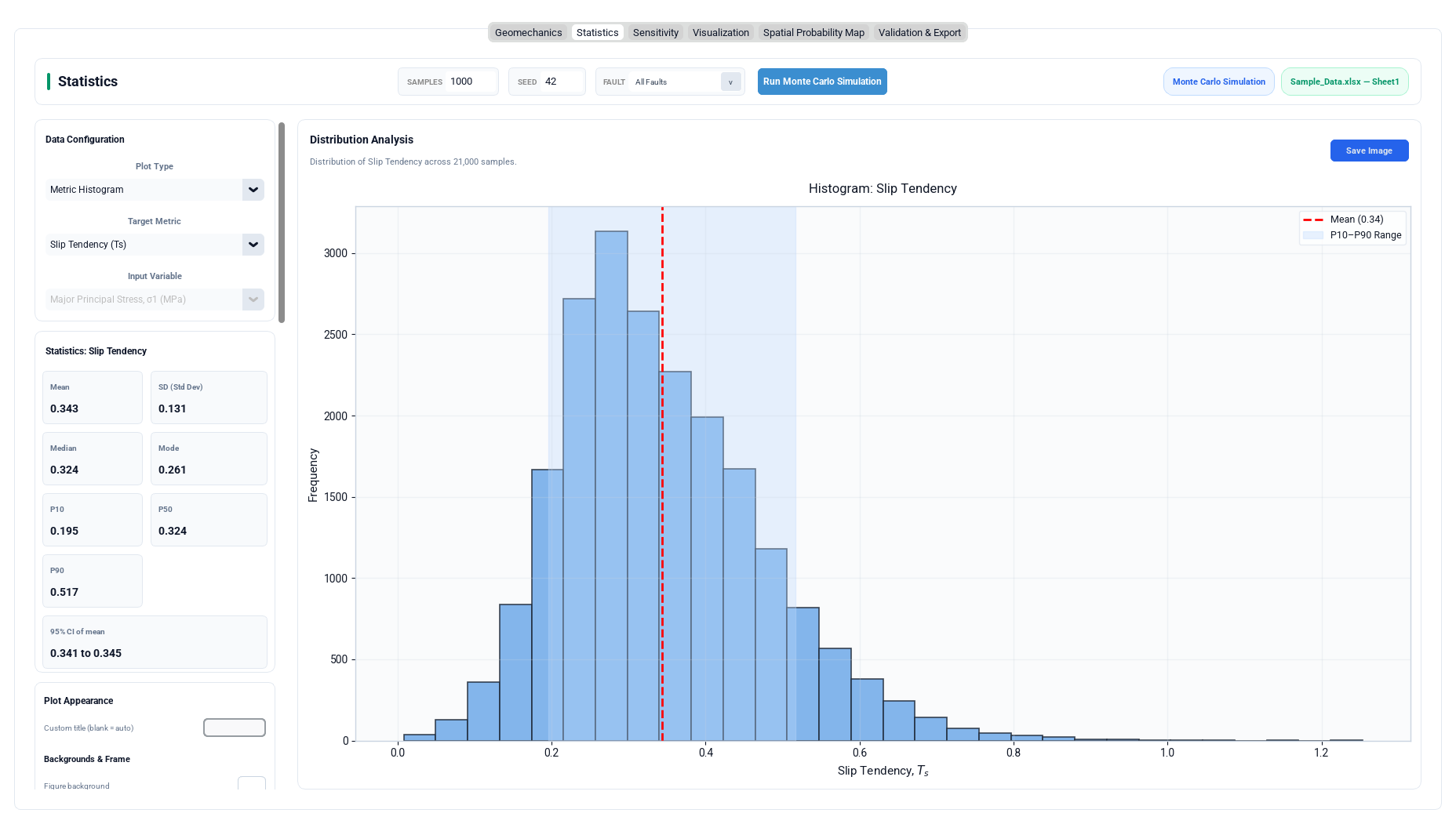
For the currently selected metric (Ts, Td, Sf, or Fs) or sampled input, the Statistics module computes and displays, in a compact grid of eight cards:

Statistic	Formula / Definition
Mean	Arithmetic mean of the finite realization values
SD (Std Dev)	Sample standard deviation, ddof = 1 (Bessel's correction)
Median	50th percentile
Mode	Most frequently occurring value after rounding to 3 decimal places
P10, P50, P90	10th, 50th (duplicate of Median), and 90th percentiles
95% CI of mean	mean ± 1.96 × SEM, where SEM = SD / √N (large-sample Normal approximation to the sampling distribution of the mean)

Two of the sampled inputs wrap, and are summarised on the circle. Fault strike is axial (period 180°: 179° and 1° are 2° apart, not 178°) and the SHmax azimuth is directional (period 360°). Neither has a meaningful arithmetic mean or standard deviation, so _input_location_and_spread() routes both through _circular_mean_and_sd(), which maps the angles onto the full circle, reduces them to their mean resultant vector, and maps the result back (Mardia and Jupp, 2000, sec. 2.2.1, 2.3.2, 2.3.4; Fisher, 1993, sec. 2.3.1):

The 180° period for strike is the standard doubling transform for axial data. Dip is a plunge confined to 0–90° and does not wrap, so it — like the stresses, friction, cohesion, and pore pressure — keeps the ordinary linear summary.

The same rule governs the P10/Mean/P90 overlay drawn on input histograms (Section 10.4). For a wrapping input the location line is the circular mean and the P10/P90 pair is taken on the angular residual about it, (θ − mean + period/2) mod period − period/2, because an ordinary quantile of a wrapping variable is fixed by where the coordinate happens to have been cut rather than by the data: on a strike sample clustered near 0° the raw P10–P90 band covered almost the entire 0–180° range while the samples themselves sat within a few degrees of the ends. When the resulting interval straddles the wrap point, the two arcs it genuinely occupies are shaded separately instead of one band running the wrong way round the circle.

Four plot types are available: Metric Histogram (with a mean reference line and a shaded P10–P90 band), Sampled Input Distribution (histogram of any single stochastic input, annotated with its mean/SD or, for orientation inputs, its mean/k), Input-Response Plot (a dual-axis scatter of the chosen output metric against a chosen input, overlaid on that input's histogram on a secondary y-axis, with an optional response-trend curve), and Probabilistic Response (Single) (a histogram of one predefined input with the response trend overlaid on a twin axis and configurable independent Y1/Y2 axis limits).

The response trend line, computed in _plot_response_trend, supports three fitting methods: Binned mean (the input range is divided into histogram-matched bins and the mean response is plotted at each bin's mean input value — a non-parametric, assumption-free summary), Linear regression (a first-degree least-squares polynomial fit), and Quadratic regression (a second-degree least-squares polynomial fit for capturing curvature in the input-response relationship).

9.2 Per-Fault Statistics

per_fault_statistics() (statistics.py) groups the realization table by fault_id and computes, for each fault, the mean, median, standard deviation, and the P05/P10/P50/P90/P95 percentiles of the selected metric, joined with a Probability of Failure column equal to the fraction of that fault's realizations with Sf ≤ 0. This per-fault breakdown underlies the Fault Uncertainty Envelope and Fault Behaviour Classification plots in the Visualization sub-tab and the Spatial Probability Map's per-fault aggregation (Section 10.5).

9.3 Global Sensitivity Analysis (Sensitivity Sub-Tab)

The Sensitivity sub-tab quantifies how strongly each of the nine stochastic inputs (σ1, σ2, σ3, pore pressure, friction, cohesion, SHmax, strike, dip) influences a chosen output metric (Ts, Td, Sf, or Fs), using two complementary regression-based measures. Before either is computed, two preparation steps apply.

Strike is folded to its axial domain. Strike is a 0–180° axial quantity, so _clean_xy() applies strike mod 180; left unfolded, the artificial discontinuity at 180°/360° corrupts both SRC and PRCC by making two nearly identical orientations numerically far apart.

Multi-fault runs are collapsed to one row per realization. Every fault in a realization is evaluated on the same sampled stress state, so the nine input columns repeat identically within a realization and only the target varies across that realization's faults. aggregate_paired_faults() therefore groups by realization and takes the mean of the inputs and the target whenever more than one fault_id is present.

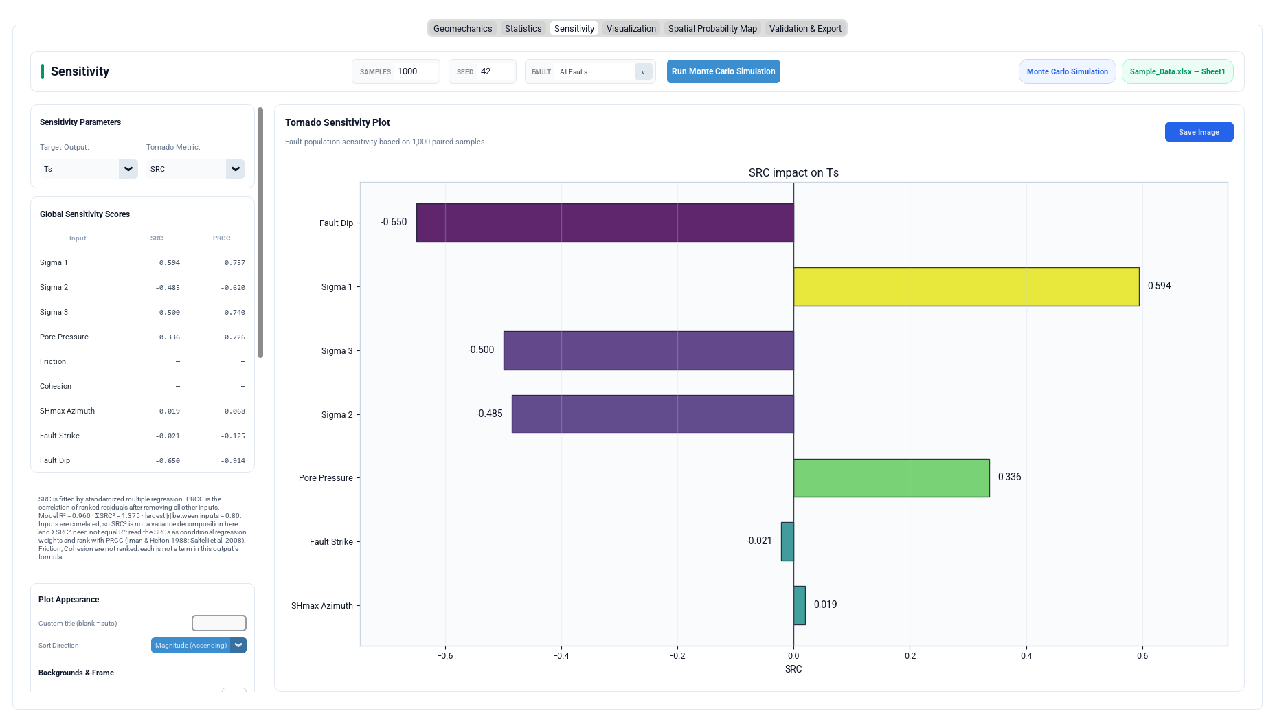
9.3.1 Standardized Regression Coefficients (SRC)

Every input column and the output column are first standardized to zero mean and unit variance (dividing by the sample SD, with inputs having zero variance safely mapped to a zero contribution rather than a division-by-zero). An ordinary least-squares multiple regression is then fit via NumPy's numpy.linalg.lstsq:

Each fitted coefficient β_i is the Standardized Regression Coefficient for input i: it measures the expected change in the output, in standard-deviation units, per one-standard-deviation change in that input, holding the (linear, additive) effect of the other inputs fixed. A run with no variation in the target raises an error rather than returning meaningless coefficients.

Squared SRCs partition the output variance — that is, they satisfy ΣSRC² = R² and may be read as variance shares — only when the inputs are mutually uncorrelated and the response is linear in them (Iman and Helton, 1988; Saltelli et al., 2008, ch. 1; Marino et al., 2008, sec. 2). Neither condition is guaranteed here: the ordered-gap sampler (Section 7.2) can draw σ1, σ2, and σ3 with strong mutual correlation. The module therefore computes and displays three diagnostics alongside the coefficients:

Diagnostic	Definition	What it tells you
Model R²	1 − SS_residual / SS_total of the standardized fit	How much of the output variance the linear model explains at all
ΣSRC²	Sum of the squared coefficients	Should equal R² if the variance-share reading is valid; any gap measures how far it is not
Largest |r| between inputs	Maximum absolute pairwise correlation among inputs that actually vary	Whether the uncorrelated-inputs precondition holds

The sidebar note prints all three on every run, and adds a warning when |r| > 0.1 and |ΣSRC² − R²| > 0.05 (read the SRCs as conditional regression weights and rank with PRCC instead), and a second warning when R² < 0.6 (the response is not well described by a linear model).

9.3.2 Partial Rank Correlation Coefficients (PRCC)

For each input, both the inputs and the output are first converted to average ranks (Spearman-style). A linear model of the remaining eight ranked inputs is fit against the ranked target input and, separately, against the ranked output; the residuals of both regressions are then correlated:

PRCC measures the monotonic association between one input and the output after removing the linear influence of every other input on both quantities, making it more robust than SRC to mild non-linearity while still requiring monotonicity in the underlying relationship.

9.3.3 Tornado Diagram

Both SRC and PRCC are tabulated in a nine-row sidebar table and one is plotted as a horizontal tornado bar chart, sorted (per the Sort Direction control) by ascending magnitude, descending magnitude, or the input's natural physical ordering. Bars can be colored by a Colormap Gradient (scaled by each coefficient's magnitude relative to the largest), by Positive/Negative sign, or with a Single Color; numeric value labels can be toggled on or off, and a zero-reference vertical line is always drawn to visually separate destabilizing from stabilizing sensitivities.

9.4 Convergence Diagnostics

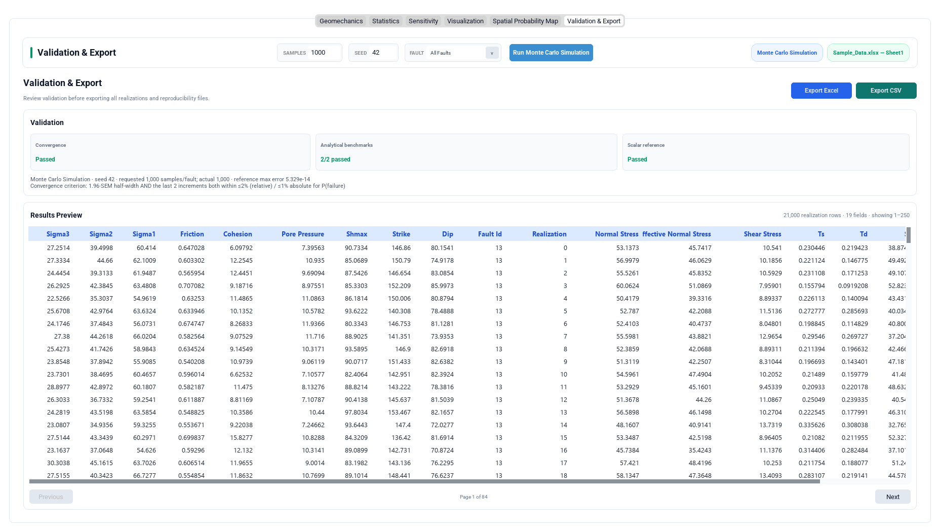
convergence_table() (validation.py) evaluates the running Ts mean, Ts P50, Ts P90, Sf mean, and probability-of-failure at a geometrically spaced sequence of nested sample-size checkpoints (between roughly 32 samples and the full requested sample count, in up to 6 steps), records the increment between successive checkpoints for each metric, and — crucially — attaches to every checkpoint a <metric>_sem column holding the Monte Carlo standard error of that estimate at that sample size.

9.4.1 Why an increment is not an error bound

A single small increment between two neighbouring sample sizes does not bound the remaining error. The nested levels form a geometric ladder, so consecutive levels differ by a factor of only about 1.5–2 and their estimates are computed from largely the same rows; two such estimates routinely agree to well inside 2% while both are still far from the limit. Measured on heavy-tailed synthetic ensembles (Pareto Ts, normal Sf, 40 independent runs per size), a final-increment-only rule reported "passed" for 10 of 40 runs at 512 realizations, and 8 of those 10 were still more than 2% away from a 400 000-realization reference. In individual runs the true remaining error reached 1.9× the increment the rule was inspecting — the increment underestimated the very error it was standing in for.

9.4.2 The two conditions

A convergence claim is a statement about the estimator's precision, so convergence_summary() requires both of the following to hold for every one of the five metrics:

Condition	Test	Rationale
Precision	The Monte Carlo half-width 1.96 × SEM at the largest level is within tolerance	Bounds how far the estimate still is from its limit (Helton and Davis, 2003; Saltelli et al., 2008, ch. 2)
Stability	The last two successive increments are both within tolerance	A single lucky step cannot certify a run; successive-refinement testing (Roache, 1998, ch. 5)

Continuous metrics use a relative tolerance; probability of failure is already a probability and uses an absolute one. A non-finite or degenerate SEM fails the precision test rather than silently satisfying it, and fewer than two checkpoint levels fails outright with an explanatory reason. Failure is reported as Not yet converged, signalling that a larger sample size is warranted for that fault/settings combination; the summary also returns the per-metric pass/fail flags, the relative increments, and the half-widths, so it is visible which metric and which condition held the run back.

9.4.3 The SEM comes from a cluster bootstrap over realizations

Every fault in a run is evaluated on the same sampled realization of the stress state, so rows that share a realization index are correlated, and an ordinary row-wise bootstrap would understate the sampling error. _cluster_bootstrap_standard_errors() therefore resamples whole realizations — the clusters — with replacement, recomputes the five statistics on each resampled pool, and takes the standard deviation across resamples (Efron and Tibshirani, 1993, ch. 8; Field and Welsh, 2007). The realizations themselves are independent draws, which is precisely what the resampling requires.

9.5 Analytical Benchmarks and Reference Comparison

In addition to the two closed-form geometric benchmark cases described in Section 6.10, a three-case reference_comparison() independently re-implements the stability equations by an entirely different route and compares them point-by-point against the vectorized NumPy implementation used for the actual Monte Carlo ensemble, on both the total- and effective-stress bases. The reference path assembles the full Cauchy stress tensor by rotation,

rather than reusing the direction-cosine expressions of Section 6.2. That independence is the point: the squared-direction-cosine shortcut is exactly what concealed the pole-convention error described in Section 6.2, so a reference built from the same shortcut could not have caught it, whereas a tensor-and-traction reference exercises the signed vector. The reference also evaluates Sf on effective normal stress unconditionally, matching the shipped definition (Section 6.7); when it instead followed the effective-stress toggle, reference_comparison(use_effective_ts=False) disagreed with the calculator by the pore pressure itself — a maximum absolute error of 12.0 MPa and "passed": False on every run.

Any discrepancy above 1×10⁻¹⁰ flags a numerical divergence between the two code paths; in normal operation this check always passes and exists as a continuous regression safeguard rather than a user-facing diagnostic.

9.6 Reproducibility Metadata

Every run's reproducibility_metadata() (validation.py) records, and later exports: an ISO-8601 UTC analysis timestamp; the sampling method and requested/actual samples per fault; the integer seed; the fault count and a SHA-256 hash of either the source file bytes or a canonical CSV serialization of the fault table (guaranteeing the exact input data can later be verified byte-for-byte); the resolved (post-truncation) distribution law for every bounded input; every configured mean/SD input parameter; the stress regime, orientation model, and per-input k values; and the installed Python, NumPy (Harris et al., 2020), pandas (McKinney, 2010), SciPy (Virtanen et al., 2020), and Matplotlib (Hunter, 2007) versions, giving a complete, audit-ready provenance record for any exported analysis.

10. Visualization Components

The Monte Carlo tab exposes five distinct plotting environments (Geomechanics, Statistics, Sensitivity, Visualization, and Spatial Probability Map), each backed by an embedded Matplotlib figure (FigureCanvasTkAgg) and each offering a Save Image button that writes a PNG at the DPI configured in the application's export settings.

10.1 Geomechanics Sub-Tab Plots

Three plot families are available via the Plot type dropdown:

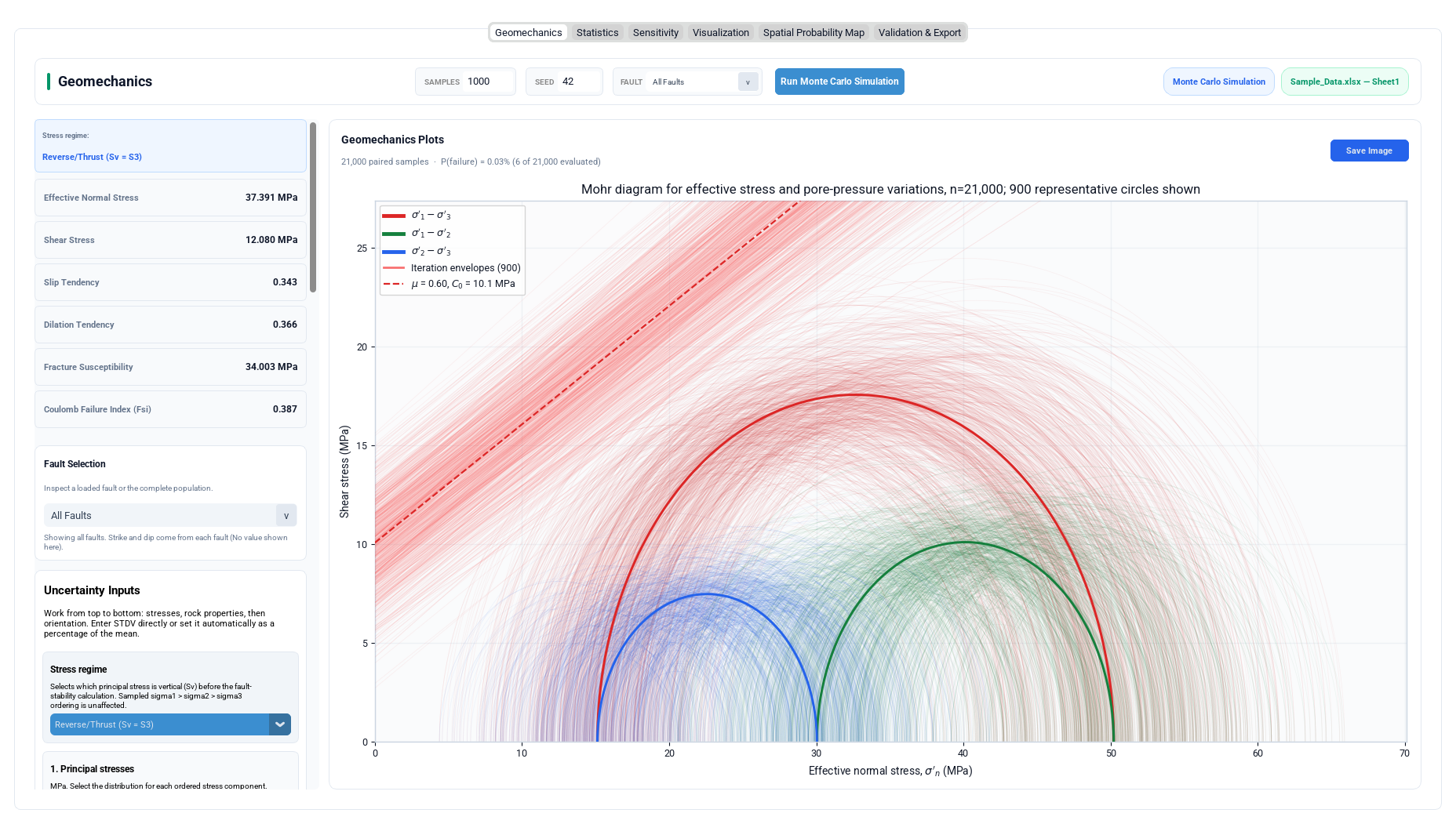
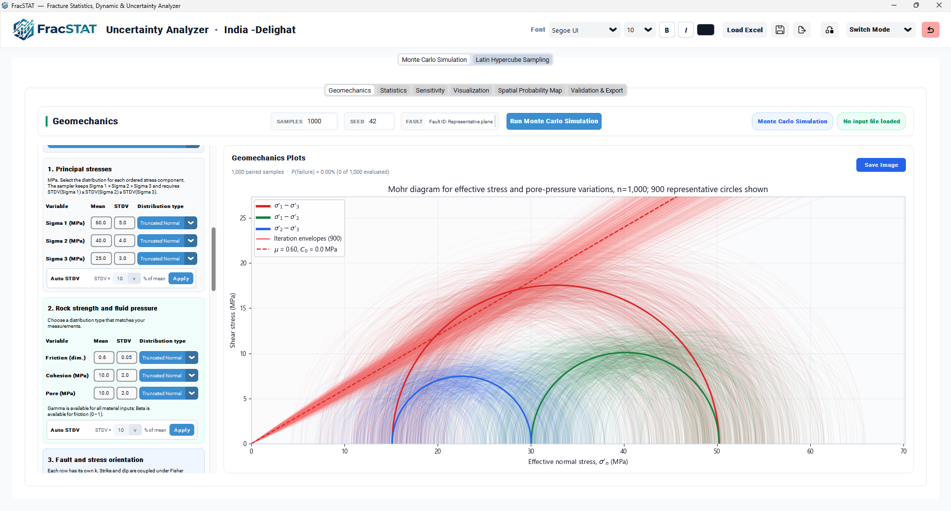
10.1.1 Mohr Uncertainty Diagrams

Draws the classical Mohr circle construction for every sampled realization (subsampled to a configurable maximum, default 900 circles, for rendering performance) as a translucent ensemble, overlaid with three bold mean circles (σ1−σ3, σ1−σ2, σ2−σ3) and the Coulomb failure envelope τ = C0 + μ·σn. When Use effective principal stresses is on, every circle is shifted left by its own realization's pore pressure (so the plot title reads "Mohr diagram for effective stress and pore-pressure variations"); an Include total-stress circles option can overlay the unshifted ensemble in grey behind the effective-stress circles for direct visual comparison of how much pore pressure moves the system toward failure.

10.1.2 Total-Stress Mohr Circles

A simplified variant that always plots on the total-stress σn axis regardless of the effective-stress toggle, useful for a stress-state overview independent of the current pore-pressure basis selection.

10.1.3 Stress Scatter

A conventional σn (or σ'n) vs. τ scatter of every realization, colored by a selectable metric (Slip tendency, Dilation tendency, or Fracture susceptibility), with optional Mohr circles (drawn at the ensemble mean principal stresses), a Coulomb failure envelope overlay, and an optional Highlight failed points marker style/color for realizations with Sf ≤ 0.

A persistent sidebar summary displays the ensemble mean of six tiles — Normal Stress (or Effective Normal Stress, matching the active basis), Shear Stress, Slip Tendency, Dilation Tendency, Fracture Susceptibility, and Coulomb Failure Index — alongside the realized Probability of Failure, recalculated live whenever the fault selection or the effective-stress toggle changes.

Figure 10.1 — Example Mohr uncertainty diagram: translucent ensemble of sampled Mohr circles, three bold mean circles, and the Coulomb failure envelope.

10.2 Statistics Sub-Tab Plots

Described in Section 9.1; the four plot types (Metric Histogram, Sampled Input Distribution, Input-Response Plot, Probabilistic Response (Single)) share a common styling card offering histogram bin count, marker/point styling, mean-line and P10–P90 range-fill styling, response-trend method/marker/color, and independent Y1/Y2 axis-limit entry fields for the dual-axis plot types.

10.3 Sensitivity Tornado Plot

Described in Section 9.3.3; supports full appearance customization (bar height/alpha/edge styling, color mode, value-label formatting) via its own Plot Appearance sidebar card.

10.4 Visualization Sub-Tab: Publication-Grade Layouts

The Visualization sub-tab is the most extensive plotting environment, offering fourteen individual Analytical Plot types plus six overall Visualization Layout modes.

Analytical Plot Type	Description
Histogram	Frequency or density histogram of the selected response metric, with optional theoretical Normal PDF overlay for goodness-of-fit inspection.
KDE	Gaussian kernel density estimate of the response metric via pandas' built-in KDE plotting.
CDF	Empirical cumulative distribution function of the response metric.
Violin Plot / Box Plot	Simultaneous distributional comparison of all four response metrics (Ts, Td, Sf, Fsi) side by side.
Ts-Td Density Contours	2-D Gaussian KDE contour map of the joint Ts/Td distribution, revealing correlated slip/dilation risk regions.
Ts-Failure Index Relationship	Scatter of Ts vs. Fs colored by Td, exposing the joint relationship between three response metrics at once.
Input-Response Plot	Scatter of any sampled input against the response metric, colored by the response value, with a twin-axis input histogram and an optional response-trend curve.
Sampled Input Distribution	Histogram of any single stochastic input in its natural (or axial, for strike) domain, with an orientation-distribution caption when applicable.
Input Distribution Diagnostics	Side-by-side density/KDE and empirical-CDF panels for one input, for detailed distribution-shape inspection.
Orientation Stereonet	Equal-area lower-hemisphere pole-point projection of every sampled fault-plane orientation, visualizing the combined strike/dip uncertainty cloud.
Probabilistic Response (Single)	One predefined input's histogram with the chosen metric's response trend on a twin axis.
Sensitivity Tornado	Standalone tornado plot using the standardized_response_sensitivity SRC-style ranking, colored by magnitude.
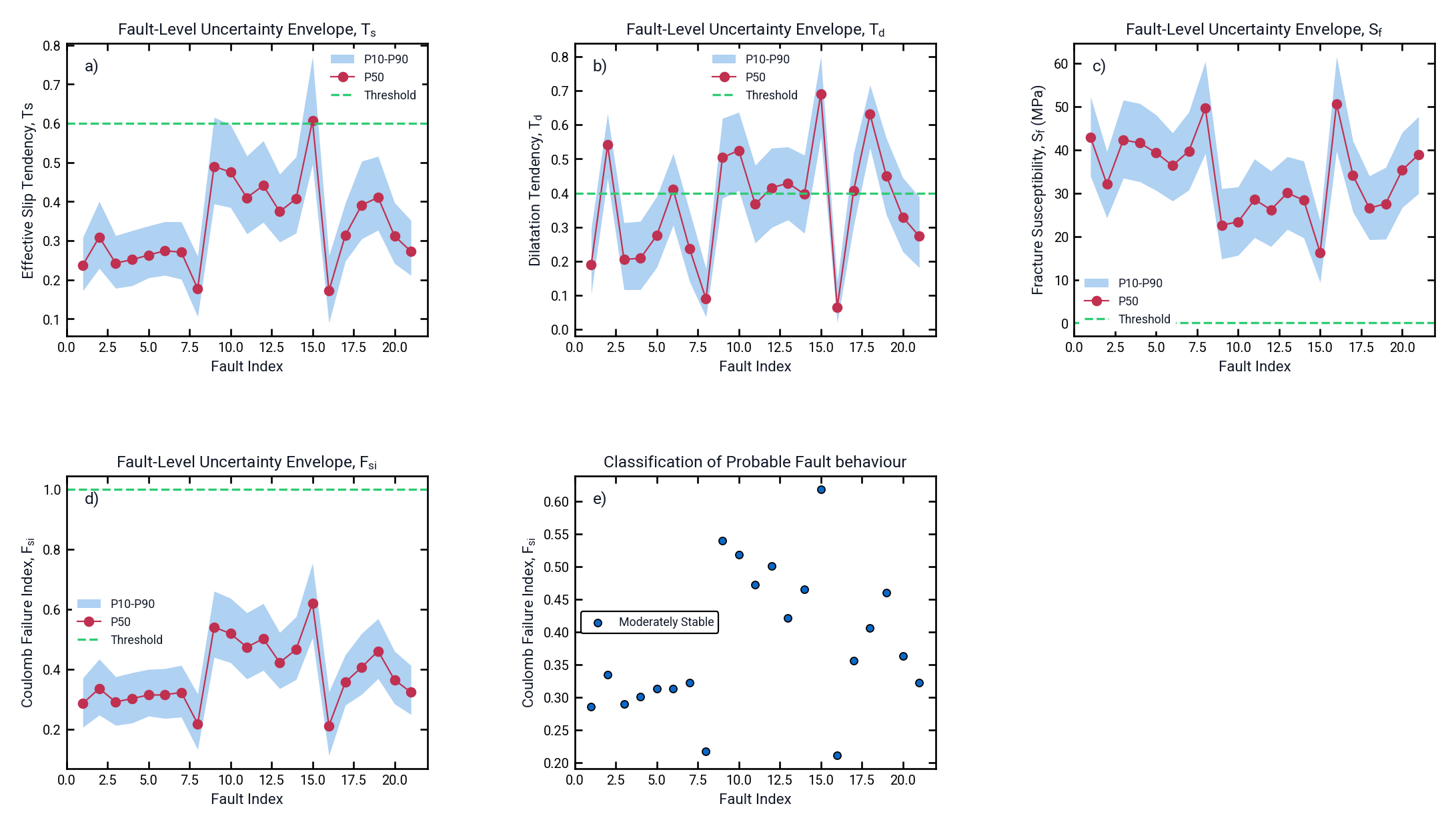
Fault Uncertainty Envelope	P10–P90 shaded band and P50 line (or, for a single fault, an error-bar point) across faults for the selected metric, with a physically meaningful threshold reference line (Ts: 0.60; Td: 0.40; Sf: 0.0; Fs: 1.00).
Fault Behaviour Classification	Scatter of per-fault median Coulomb Failure Index, color/marker-coded into "Moderately Stable" (Fs P50 < 0.80) and "Critically Stressed" (Fs P50 ≥ 0.80) classes.

Visualization Layout Mode	Description
Single Analytical Plot	Displays exactly one of the fourteen plot types above, full-size.
Four-Panel Analysis Dashboard	A 2×2 grid in which each of the four panels independently selects any of the fourteen plot types, sharing the current response metric and input parameter.
Input Parameter Distributions	A fixed 2×4 grid showing all eight sampled physical inputs' distributions simultaneously.
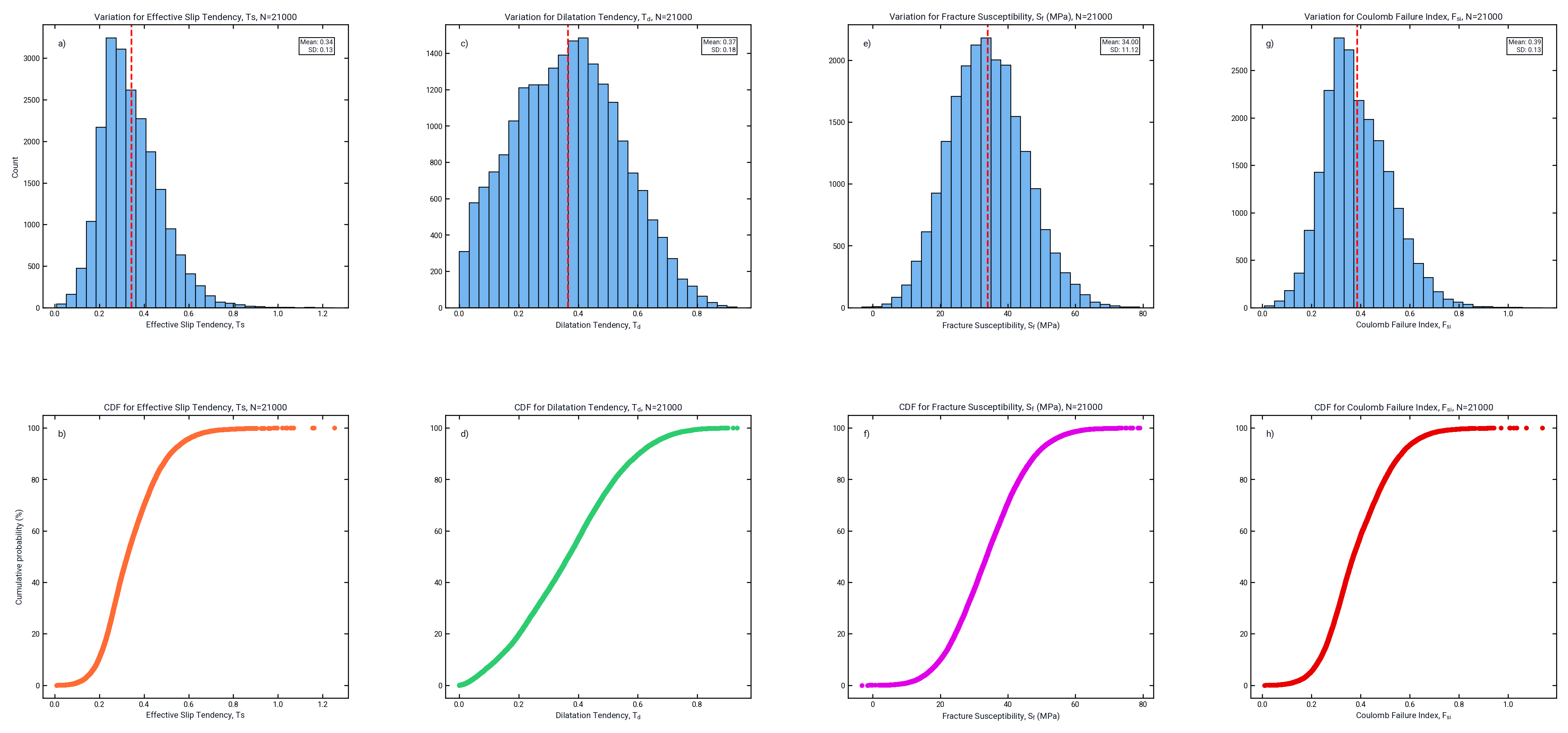
Response Metric Distributions	A fixed 2×4 grid: histogram (top row) and CDF (bottom row) for each of the four response metrics.
Probabilistic Response Analysis	A fixed 3×3 grid: eight input-vs-response panels (one per stochastic input) plus a ninth sensitivity-tornado panel for the selected metric.
Fault-Level Uncertainty Envelopes	A fixed 2×3 grid of Ts/Td/Sf/Fs envelopes plus the Fault Behaviour Classification scatter, each with independently stored Y-axis limits.

Two statistical overlay checkboxes — Overlay KDE Curve and Overlay P10/Mean/P90 — apply uniformly across every eligible plot type and layout mode, adding a smoothed density curve and/or a shaded interquantile band with mean-line annotation. On the two wrapping inputs (strike, period 180°; SHmax azimuth, period 360°) the band and mean line are computed on the circle rather than on the line, and a band that straddles the wrap point is drawn as the two arcs it actually occupies — see Section 9.1 for the formulae and the measured error the linear version produced. A Full-Screen viewer (opened via the monitor icon) reproduces the entire toolbar in a dedicated always-on-top window with its own compact selector row, letting a user present or inspect a plot at full display resolution while retaining every interactive control.

10.5 Spatial Probability Map Sub-Tab

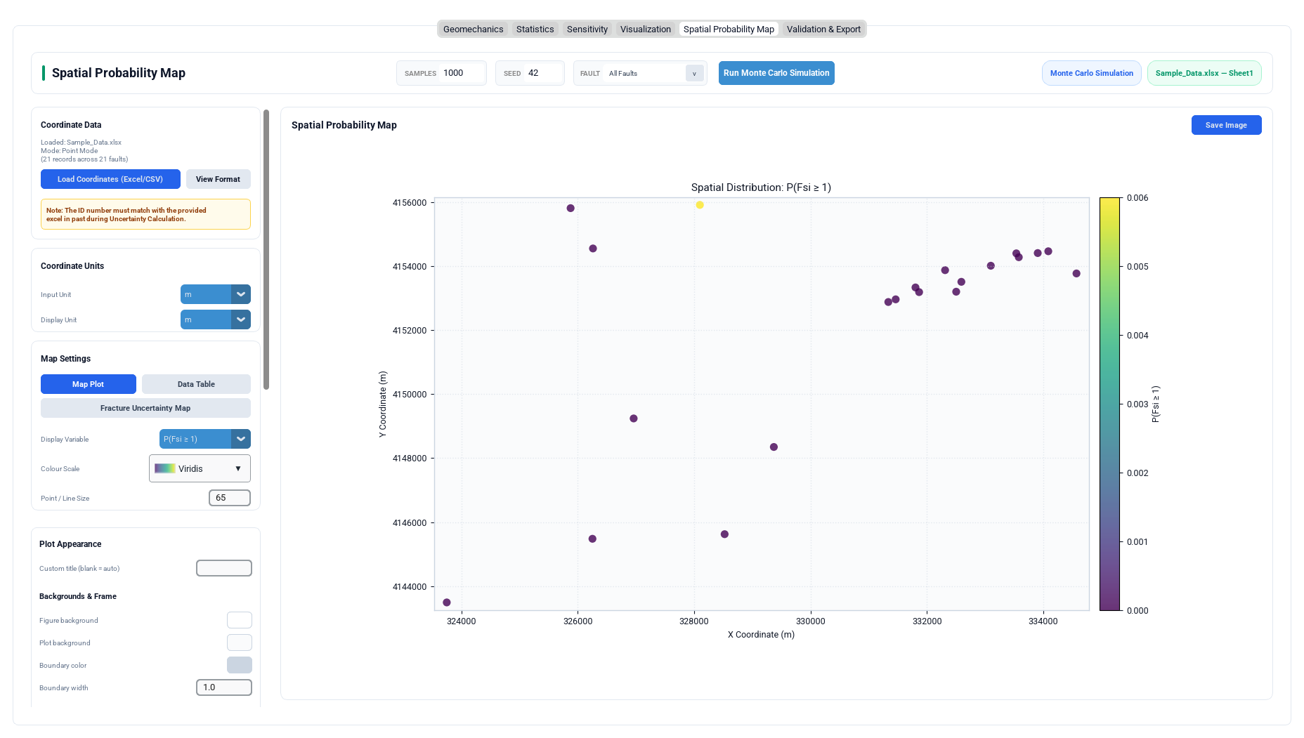
This sub-tab is unique among the six in requiring a second, independently loaded data source: a coordinate file (Excel/CSV) mapping each fault_id to either a single X/Y point or an X1/Y1–X2/Y2 trace segment, matched against the Monte Carlo results by ID. Column-alias detection accepts numerous header variants (Easting/Northing, bracketed unit suffixes such as "X [km]", etc.) and automatically infers the coordinate unit from the header text when possible.

Once coordinates are loaded, the module aggregates the realization population per fault_id into Fsi (mean Coulomb Failure Index), P10, P50, P90, and P(Fsi ≥ 1) (the fraction of realizations exceeding the failure threshold), computes an Uncertainty_Width = P90 − P10 metric, and offers three views:

• Map Plot — a georeferenced scatter (point mode) or line-collection (trace mode) map colored by the selected metric, with a coordinate-unit conversion pipeline (km/m/cm/mm), optional fault-ID text labels, and a positionable colorbar.
• Data Table — a scrollable tabular preview of the merged coordinate/probability data (capped at 500 rows for UI responsiveness), exportable to Excel or CSV independently of the main Validation & Export sub-tab.
• Fracture Uncertainty Map — a horizontal bar chart ranking every fault by Uncertainty_Width, auto-sized (up to 60 inches tall) so that large fault populations remain legible without overlapping labels, with an optional numeric value annotation on each bar.

11. Advanced Features

11.1 Move Layout Elements (Edit Mode)

A shared workspace-level Edit Mode toggle (in the WorkspaceHeaderMixin, invoked identically across all six sub-tabs) makes every plot legend draggable and enables free repositioning of plot axes by mouse drag. When engaged, matplotlib's constrained/tight layout engine is disabled for the affected figure (figure.set_constrained_layout(False)) so that manually dragged axis positions are not immediately overridden on the next redraw; twinned axes (e.g. a histogram's count axis paired with a response-trend axis) are detected by comparing bounding-box positions and moved together as a group so overlays stay aligned.

11.2 Manual Plot Pixel Sizing

Every sub-tab's Plot Appearance card exposes a Plot size (px) width/height control pair with an Apply Plot Size button (plot_size.apply_plot_pixel_size). This resizes the embedded Qt canvas widget directly (clamped to the range 240–4096 px per dimension), letting a user produce a figure at an exact pixel footprint suitable for a specific publication template or presentation slide, independent of the surrounding window size.

11.3 Custom Typography and Font Propagation

The shared workspace header's font family, size, weight, italic, and color controls (in uncertainty_app.py) are applied not only to the surrounding Qt UI but are actively re-applied to every Matplotlib artist — titles, axis labels, tick labels, legend text, and colorbar labels — across every registered figure in every sub-tab (_apply_uncertainty_figure_fonts), ensuring visual consistency between the on-screen application chrome and the exported plot images.

11.4 Worksheet Selection for Multi-Sheet Workbooks

Described in Section 4.1; this is implemented as a lightweight modal dialog rather than a silent "first sheet wins" default, preventing a common source of user error when a spreadsheet contains multiple related tabs (e.g. a raw-data sheet alongside a summary sheet).

11.5 Cross-Fault Result Caching and Restoration

Described further in Section 12.1; from the user's perspective, this surfaces as near-instantaneous switching between the All Faults view and any individual fault once at least one run has completed, along with a status-bar message ("Restored previously simulated results for …") confirming that cached data, not a fresh simulation, is being displayed.

11.6 Session Save/Restore and Cross-Module Isolation

The complete Monte Carlo session — loaded input file, every sidebar setting, and (implicitly, via autosave) the most recent results — is persisted per-project and reloaded automatically when the project is reopened, independent of whatever Static or Dynamic Analyzer state exists for the same project (Section 8.5).

12. Performance Optimization

12.1 Fault-Level Result Caching

fault_result_cache is a dictionary keyed by fault-selection label, storing the (results, validation_report) tuple produced by every completed run. When the user selects an individual fault that has no direct cache entry but an All Faults run has already been completed, _cached_fault_results_from_all_fault_run() slices that population by fault_id, recomputes only the lightweight convergence table and metadata for that subset, and caches the result — avoiding an entirely new (and computationally redundant) simulation. Loading a new input file or changing the sampling settings invalidates this cache, since a newly loaded source may reuse an existing Fault ID label that would otherwise return stale results.

12.2 Active-Tab-Only Redrawing

refresh_active_module() redraws only the Matplotlib figure(s) belonging to the currently visible module sub-tab; the other five sub-tabs' plots are refreshed lazily, the first time each becomes visible after new results arrive. This avoids six simultaneous, expensive Matplotlib redraws (including scatter re-rendering, colorbar reconstruction, and legend layout) every time a simulation completes or a fault is switched.

12.3 Debounced Appearance-Setting Redraws

Because many appearance controls (color swatches, sliders, dropdowns) can fire several rapid variable-write events in a single user interaction (e.g. a color picker emitting intermediate values while being dragged, or Reset to Defaults setting ~30 variables at once), every sub-tab coalesces these bursts into a single scheduled redraw roughly 60–80 milliseconds after the last change, using the after()/after_cancel() scheduling primitives. This eliminates visible flicker and avoids redundant full figure.clear()-and-rebuild cycles.

12.4 Threaded I/O and Computation

File loading (Section 4), coordinate loading for the Spatial Probability Map (Section 10.5), and the Monte Carlo sampling/validation pipeline itself (Section 8.2) all execute on background daemon threads, with results marshaled back to the Qt main thread via widget.after(0, callback). This keeps the application's event loop responsive — including allowing the Cancel control to be clicked — throughout potentially long-running operations.

12.5 Vectorized Stability Calculation

calculate_fault_stability() operates on entire NumPy arrays of realizations at once (rather than looping in Python per realization), so the per-realization cost of Equations 6.1–6.11 is amortized across the whole ensemble via compiled array operations — essential for keeping sample sizes up to 100,000 responsive.

12.6 Bounded Mohr-Circle Rendering

The Geomechanics sub-tab's Mohr uncertainty diagrams cap the number of individually rendered circles (Max. displayed circles, default 900) by selecting evenly spaced representative realizations from the full ensemble via a linear index subsample, rather than rendering one Matplotlib LineCollection segment per realization — preventing the plot from becoming sluggish or visually saturated at large sample sizes while preserving a representative visual impression of the full distribution.

12.7 Scrollable Auto-Sizing for Large Fault Populations

The Fracture Uncertainty Map (Section 10.5) dynamically grows its figure height (up to 60 inches) in proportion to the number of faults, embedded inside a scrollable Qt frame, only recalculating this size when the fault count itself changes (not on every cosmetic appearance edit) — avoiding both label overlap for large fault populations and unnecessary canvas reconfiguration during routine styling adjustments.

13. Practical Examples

13.1 Example 1 — Single Representative Fault Screening

Scenario: A geomechanical analyst has measurement uncertainty on a single, poorly constrained fault plane (Strike 45° ± 5°, Dip 60° ± 5°) and wants a rapid screening estimate of reactivation risk under current reservoir stress conditions, without loading a spreadsheet.

1. Open the Monte Carlo Simulation tab without loading any input file; the sampler falls back to the built-in representative plane (Section 4.3).
2. In Geomechanics, set the Stress Regime to Reverse/Thrust (S_v = S3), enter the site's principal-stress means/SDs and distributions, and confirm Friction, Cohesion, and Pore Pressure means reflect the best available core or offset-well data.
3. Set SAMPLES to 5000 and SEED to any fixed integer for reproducibility, then click Run Monte Carlo Simulation.
4. Inspect the Geomechanics sidebar's Probability of Failure tile and the Mohr uncertainty diagram; a cluster of sampled circles crossing the Coulomb envelope indicates meaningful reactivation risk even if the mean case appears stable.
5. Open Sensitivity to identify which input (e.g. pore pressure or friction) contributes most to the spread in Fsi, focusing further data-acquisition effort on that parameter.

13.2 Example 2 — Population-Level Injection Risk Screening

Scenario: A CO₂-injection or produced-water-disposal operator has a spreadsheet of 40 mapped faults (with Strike, Dip, and per-fault Sigma columns) and needs to rank faults by injection-induced reactivation risk under an anticipated pore-pressure increase.

1. Load the fault spreadsheet via the workspace header's Load Excel control; confirm the Analysis columns selected dialog correctly matched every expected column.
2. In Geomechanics, set FAULT to All Faults, enable Use effective principal stresses, and set the Pore Pressure mean to the anticipated post-injection value (with an SD reflecting monitoring/interpretation uncertainty).
3. Run the simulation with a moderate sample size (e.g. 2000 per fault) suitable for 40 faults × 2000 = 80,000 total realizations.
4. In Visualization, select the Fault-Level Uncertainty Envelopes layout to view all faults' Ts/Td/Sf/Fs P10–P90 envelopes and the Fault Behaviour Classification scatter simultaneously.
5. Load the corresponding coordinate file in Spatial Probability Map and select P(Fsi ≥ 1) as the Display Variable to produce a map directly identifying the highest-risk fault locations for stakeholder communication.
6. Export the full validated result set (Section 9.6) via Validation & Export → Export Excel for the permanent project record.

13.3 Example 3 — Comparing Von Mises and Fisher 3D Orientation Models

Scenario: An analyst wants to test whether treating strike and dip uncertainty as coupled (Fisher 3D) rather than independent (Von Mises) materially changes the predicted probability of failure for a critically oriented fault.

1. Run the simulation once with Orientation Distribution set to Von Mises and a fixed seed, recording the resulting Probability of Failure and Ts P10–P90 range from the Statistics sub-tab.
2. Switch Orientation Distribution to Fisher 3D (leaving every other setting, including the seed, unchanged) and re-run.
3. Compare the two Ts histograms side by side (Statistics sub-tab) and the two Orientation Stereonet plots (Visualization sub-tab) to visualize how the coupled Fisher model reshapes the sampled orientation cloud relative to the independent Von Mises model.

14. Geological and Engineering Interpretation

14.1 Reading Slip Tendency (Ts)

A realization's Ts should be compared against an appropriate frictional threshold; Byerlee's Law suggests typical crustal rock friction coefficients cluster near μ ≈ 0.6–0.85, so Ts values approaching or exceeding roughly 0.6 in the sampled population indicate that a meaningful fraction of plausible stress/strength combinations places the fault near or past frictional failure. The Monte Carlo population view is essential here: a deterministic mean-case Ts below the threshold can still coexist with a substantial P90 tail above it, meaning failure is a real (if not certain) possibility rather than a remote one.

14.2 Reading Dilation Tendency (Td)

High Td (approaching 1) identifies fault or fracture orientations most favorably aligned for hydraulic opening (dilation) under the current stress field — geologically significant for identifying preferential fluid-flow pathways, potential conduits for fault-controlled mineralization, or, in an injection context, faults most susceptible to opening-mode reactivation rather than pure frictional slip.

14.3 Reading Fracture Susceptibility (Sf) and the Coulomb Failure Index (Fsi)

Sf provides a physically interpretable stress margin in MPa — the amount by which normal stress would need to change (holding shear stress, friction, and cohesion fixed) to bring the fault exactly onto the failure envelope. Fsi, being dimensionless and normalized so that 1.0 always marks the failure envelope regardless of the specific friction/cohesion values, is generally the preferred metric for comparing relative risk across faults with different strength properties, as is done in the Fault Behaviour Classification plot's fixed 0.80 Fsi threshold for the "Critically Stressed" category.

14.4 Effect of the Effective-Stress Toggle on Interpretation

Disabling Use effective principal stresses produces a conservative, total-stress-only assessment appropriate for a baseline geological characterization where current pore pressure is either unknown or intentionally excluded from the stability question. Enabling it is essential whenever the analysis question specifically concerns fluid-pressure-driven reactivation (injection, depletion, or natural pore-pressure evolution), since Terzaghi effective-stress theory is the physically correct basis for assessing frictional failure in a fluid-saturated rock mass.

14.5 Stress Regime Selection and Its Geological Basis

The stress-regime selector (Sections 5.1, 6.4) should be set according to independent evidence for the tectonic regime at the site of interest (e.g. from World Stress Map compilations, borehole breakout analysis, or regional structural geology), not chosen arbitrarily; an incorrect regime assignment will systematically misplace the vertical stress within the fault-normal-stress calculation and can materially bias every downstream metric.

14.6 Orientation Model Selection and Its Geological Basis

Von Mises independent sampling is appropriate when strike and dip uncertainty genuinely originate from separate, uncorrelated sources (for example, strike picked from a seismic horizon and dip estimated separately from an image log in a different well). Fisher 3D coupled sampling is appropriate whenever the orientation uncertainty is inherently a single combined angular measurement uncertainty (for example, a single planar feature interpreted from one borehole-image or outcrop measurement), since the Fisher distribution correctly represents uncertainty as a cone around one 3-D pole direction rather than as two independent linear wobbles.

15. Implementation Notes

15.1 Software Dependencies

Library	Role in the Monte Carlo Tab
NumPy	Random number generation (Generator API), vectorized array arithmetic for stability calculations and distribution transforms.
SciPy (scipy.stats)	Probability-distribution quantile functions (norm, truncnorm, lognorm, beta, gamma, vonmises) and the Latin Hypercube QMC engine (used by the sibling LHS tab).
pandas	Tabular fault data ingestion, DataFrame-based realization storage, groupby-based per-fault statistics, and CSV/Excel export.
Matplotlib	All embedded plotting (Figure/FigureCanvasTkAgg), including Mohr circles, scatter plots, tornado charts, contour maps, and the stereonet projection.
PySide6 via ui_common.qtk (ctk)	The entire GUI control layer — tabs, entries, dropdowns, sliders, checkboxes, and scrollable frames.
openpyxl (via pandas.ExcelWriter)	Multi-sheet Excel export in the Validation & Export sub-tab.

15.2 Numerical Stability Safeguards

• The shear-stress radicand in Equation 6.5 is clamped to a minimum of zero to prevent NaN results from floating-point rounding near zero shear.
• Every distribution transform in sample_scalar() clips its unit-uniform input to the open interval (1×10⁻¹², 1−1×10⁻¹²) before applying an inverse-CDF, preventing infinite quantile values at the extremes.
• Denominators in Ts, Td, Sf, and Fs are guarded with explicit validity masks (e.g. calculation_normal > 0, friction_valid, dilation_valid) so that an invalid realization yields a reported missing value rather than a divide-by-zero exception or a silently wrong number.
• The principal-stress gap-variance construction (Equation 7.3) clamps its radicand to zero rather than allowing a negative variance under a (validated-against) inverted SD ordering.

15.3 Threading Model Summary

All Qt widget mutations occur exclusively on the main thread; every background thread (file loading, simulation, coordinate loading) communicates results back via widget.after(0, callback), and every long-running loop checks a shared threading.Event for cooperative cancellation at well-defined checkpoints rather than being forcibly terminated.

15.4 Data Model Summary

The canonical realization table produced by generate_samples() is a single pandas DataFrame with one row per (fault, realization) pair, carrying columns for every sampled input (sigma1–sigma3, friction, cohesion, pore_pressure, shmax, strike, dip), the derived stability outputs (normal_stress, effective_normal_stress, shear_stress, Ts, Td, Sf, Fs, failure), and identifying columns (fault_id, realization). Provenance and configuration are attached as DataFrame .attrs metadata (stress_regime, distribution_settings, configured_distributions, effective_distributions, orientation_distribution, orientation_k_by_input, use_effective_ts, slip_tendency_stress_basis) rather than as additional data columns, keeping the tabular export clean while preserving full reproducibility.

16. Limitations

Limitation	Description
Idealized fault geometry	The underlying stability physics assumes planar, non-intersecting fault surfaces with spatially uniform stress and strength properties per realization; fault-zone heterogeneity, curvature, and stress perturbation near fault tips are not modeled.
Independent inputs	Inputs other than fault orientation and the ordered principal stresses are assumed statistically independent of one another; correlated uncertainty between, for example, cohesion and friction (common in some laboratory-derived strength envelopes) is not natively supported and would require an external pre-transformation of the input distributions. Note that the ordered-gap sampler (Section 7.2) does induce correlation among σ1, σ2, and σ3, which is why the SRC diagnostics of Section 9.3.1 are reported.
Linear failure criterion	The Mohr–Coulomb failure criterion is linear in normal stress; non-linear (e.g. Hoek–Brown or Barton–Bandis) failure envelopes are not implemented.
First-order sensitivity measures	Sensitivity coefficients (SRC, PRCC) are regression-based, global, first-order measures; they do not capture higher-order interaction effects between inputs. Squared SRCs are a variance decomposition only when the inputs are uncorrelated and the response is linear, so the reported R², ΣSRC², and largest input |r| must be read alongside the tornado diagram; where they disagree, rank with PRCC.
Convergence is a heuristic	The two-condition convergence criterion of Section 9.4 (precision: 1.96 × SEM within 2% / 1 percentage point; stability: two successive increments within tolerance) is a practical stopping rule applied to five named metrics only. A run reported as "Passed" does not guarantee that every downstream statistic — an extreme tail percentile, a per-fault probability — has converged to the same accuracy.
Fracture susceptibility is always effective-stress	Sf is a sustainable pore-pressure increase and is therefore computed on σ'n = σn − Pp regardless of the effective-stress toggle (Section 6.7). There is no total-stress form of Sf, so the toggle changes Ts, Td, and Fs but deliberately leaves Sf and the failure flag derived from it untouched. It is undefined (NaN) when σ'n ≤ 0 or μ ≤ 0.
Regime handling is a permutation of inputs	The stress calculator hard-codes one geometric assignment (σ1 along SHmax, σ3 vertical). Regimes are realised by permuting which sampled magnitude enters each slot (Section 6.4), not by re-deriving the geometry, and an unrecognised regime string silently falls back to reverse/thrust. Inside the calculator the argument names denote slots, not global maximum and minimum.
Cluster bootstrap resample count	Standard errors come from 200 bootstrap resamples of whole realizations, reduced to 60 above 20,000 rows for runtime (Section 9.4.3); the SEM is itself a Monte Carlo estimate with its own sampling noise, and it is returned as NaN when a checkpoint contains fewer than two realizations.
Wrapping inputs summarised on the circle only where implemented	Strike (period 180°) and the SHmax azimuth (period 360°) receive circular means, dispersions, and overlay bands (Section 9.1), and strike is folded modulo 180° before sensitivity fitting. Other circular diagnostics — a formal concentration test, a Rayleigh or Watson uniformity statistic on the sampled orientations — are not computed.
Exact-ID coordinate matching	The Spatial Probability Map requires exact string-matched Fault IDs between the Monte Carlo input spreadsheet and the separately loaded coordinate file; no fuzzy or coordinate-based automatic matching is performed.
Sample-size cap	Maximum sample size is capped at 100,000 realizations per fault by UI validation; very large multi-fault populations (many faults × large sample counts) are bounded primarily by available system memory and interactive redraw performance rather than by an explicit software limit.
Single-parameter Fisher coupling	The Fisher 3D orientation model couples strike and dip using a single shared concentration parameter (from the Strike row); it does not support independently specified strike and dip concentrations within the coupled model.
Truncated-normal moment constraints	A truncated normal on [l, u] cannot have sd above (u − l)/√12 (the limit is lower away from the midpoint), and on [0, ∞) cannot have sd/mean ≥ 1. Such requests raise rather than silently changing moments (Section 7.4). Consider Lognormal or Gamma for positive unbounded inputs, or Beta or a feasible Uniform law for friction on [0,1]; these alternatives have their own support constraints.

17. References

Sources are listed alphabetically within each group. In-text citations throughout this page link to the corresponding entry below.

17.1 Rock Mechanics, Effective Stress and Fault Stability

• Byerlee, J. (1978). Friction of rocks. Pure and Applied Geophysics, 116(4–5), 615–626. https://doi.org/10.1007/BF00876528
• Ferrill, D. A., & Morris, A. P. (2003). Dilational normal faults. Journal of Structural Geology, 25(2), 183–196. https://doi.org/10.1016/S0191-8141(02)00029-9
• Hubbert, M. K., & Rubey, W. W. (1959). Role of fluid pressure in mechanics of overthrust faulting. Geological Society of America Bulletin, 70(2), 115–166. https://doi.org/10.1130/0016-7606(1959)70[115:ROFPIM]2.0.CO;2
• Jaeger, J. C., Cook, N. G. W., & Zimmerman, R. W. (2007). Fundamentals of Rock Mechanics (4th ed.). Blackwell Publishing, Oxford. ISBN 978-0-632-05759-7. (Mohr–Coulomb failure theory, effective stress.)
• Mildren, S. D., Hillis, R. R., & Kaldi, J. (2002). Calibrating predictions of fault seal reactivation in the Timor Sea. The APPEA Journal, 42(1), 187–202. https://doi.org/10.1071/AJ01011
• Morris, A., Ferrill, D. A., & Henderson, D. B. (1996). Slip-tendency analysis and fault reactivation. Geology, 24(3), 275–278. https://doi.org/10.1130/0091-7613(1996)024<0275:STAAFR>2.3.CO;2
• Streit, J. E., & Hillis, R. R. (2004). Estimating fault stability and sustainable fluid pressures for underground storage of CO₂ in porous rock. Energy, 29(9–10), 1445–1456. https://doi.org/10.1016/j.energy.2004.03.078
• Terzaghi, K. (1943). Theoretical Soil Mechanics. John Wiley & Sons. https://doi.org/10.1002/9780470172766
• Zoback, M. D. (2007). Reservoir Geomechanics. Cambridge University Press. https://doi.org/10.1017/CBO9780511586477

17.2 Probability Distributions and Directional Statistics

• Fisher, R. A. (1953). Dispersion on a sphere. Proceedings of the Royal Society A, 217(1130), 295–305. https://doi.org/10.1098/rspa.1953.0064
• Fisher, N. I. (1993). Statistical Analysis of Circular Data. Cambridge University Press. https://doi.org/10.1017/CBO9780511564345 (Circular mean and circular standard deviation, sec. 2.3.1.)
• Johnson, N. L., Kotz, S., & Balakrishnan, N. (1994). Continuous Univariate Distributions, Vol. 1 (2nd ed.). John Wiley & Sons. ISBN 978-0-471-58495-7. (Sec. 13.10: moments of the truncated normal distribution.)
• Mardia, K. V., & Jupp, P. E. (2000). Directional Statistics. John Wiley & Sons. https://doi.org/10.1002/9780470316979 (Von Mises and spherical/Fisher distribution theory; circular mean and dispersion, sec. 2.2.1 and 2.3.4; the doubling transform for axial data, sec. 2.3.2.)

17.3 Sampling, Sensitivity and Convergence

• Efron, B., & Tibshirani, R. J. (1993). An Introduction to the Bootstrap. Chapman & Hall. https://doi.org/10.1007/978-1-4899-4541-9 (Ch. 8: bootstrapping clustered and non-iid data.)
• Field, C. A., & Welsh, A. H. (2007). Bootstrapping clustered data. Journal of the Royal Statistical Society: Series B, 69(3), 369–390. https://doi.org/10.1111/j.1467-9868.2007.00593.x
• Helton, J. C., & Davis, F. J. (2003). Latin hypercube sampling and the propagation of uncertainty in analyses of complex systems. Reliability Engineering & System Safety, 81(1), 23–69. https://doi.org/10.1016/S0951-8320(03)00058-9
• Iman, R. L., & Conover, W. J. (1982). A distribution-free approach to inducing rank correlation among input variables. Communications in Statistics — Simulation and Computation, 11(3), 311–334. https://doi.org/10.1080/03610918208812265
• Iman, R. L., & Helton, J. C. (1988). An investigation of uncertainty and sensitivity analysis techniques for computer models. Risk Analysis, 8(1), 71–90. https://doi.org/10.1111/j.1539-6924.1988.tb01155.x
• Marino, S., Hogue, I. B., Ray, C. J., & Kirschner, D. E. (2008). A methodology for performing global uncertainty and sensitivity analysis in systems biology. Journal of Theoretical Biology, 254(1), 178–196. https://doi.org/10.1016/j.jtbi.2008.04.011
• McKay, M. D., Beckman, R. J., & Conover, W. J. (1979). A comparison of three methods for selecting values of input variables in the analysis of output from a computer code. Technometrics, 21(2), 239–245. https://doi.org/10.2307/1268522
• Roache, P. J. (1998). Verification and Validation in Computational Science and Engineering. Hermosa Publishers, Albuquerque. ISBN 978-0-913478-08-0. (Ch. 5: successive-refinement stability as a convergence test.)
• Saltelli, A., Ratto, M., Andres, T., Campolongo, F., Cariboni, J., Gatelli, D., Saisana, M., & Tarantola, S. (2008). Global Sensitivity Analysis: The Primer. John Wiley & Sons. https://doi.org/10.1002/9780470725184

17.4 Software

• Harris, C. R., Millman, K. J., van der Walt, S. J., Gommers, R., Virtanen, P., Cournapeau, D., … Oliphant, T. E. (2020). Array programming with NumPy. Nature, 585(7825), 357–362. https://doi.org/10.1038/s41586-020-2649-2
• Hunter, J. D. (2007). Matplotlib: A 2D graphics environment. Computing in Science & Engineering, 9(3), 90–95. https://doi.org/10.1109/MCSE.2007.55
• McKinney, W. (2010). Data structures for statistical computing in Python. In Proceedings of the 9th Python in Science Conference (pp. 56–61). https://doi.org/10.25080/Majora-92bf1922-00a
• Virtanen, P., Gommers, R., Oliphant, T. E., Haberland, M., Reddy, T., Cournapeau, D., … van Mulbregt, P. (2020). SciPy 1.0: fundamental algorithms for scientific computing in Python. Nature Methods, 17(3), 261–272. https://doi.org/10.1038/s41592-019-0686-2