Dynamic Mohr Tab
Located at dynamic_analyzer/tabs/dynamic_mohr_tab.py, the Mohr Tab
(implemented as the mixin class MohrTab) is one of six coordinated views inside the
Dynamic Analyzer workspace, alongside the Map, Rose, Stereonet, Table, and Method tabs. It renders
the classical Mohr circle construction together with a linear Mohr–Coulomb failure envelope,
and overlays every loaded fracture segment or fracture plane as a stress point ("pole") on that
diagram, letting the analyst see at a glance how close each fracture sits to frictional failure
under a user-specified in-situ stress tensor, pore pressure, and Mohr–Coulomb strength
parameters.
The tab consumes the per-segment results table produced by the calculation engine
(core/calculator.py) after a Static or Dynamic Analyzer data source has been loaded
and a stress state entered in the sidebar. It performs no stress resolution itself — it
visualizes the already-computed effective normal stress, shear stress, slip tendency, dilation
tendency, fracture susceptibility, and critical-stress flag for every segment, and additionally
computes an independent continuous stress-tendency field over every possible plane orientation
for background shading.
On this page
- 1. Purpose and Scope
- 2. Interface Overview
- 3. Data Input
- 4. Settings and Controls
- 5. Mathematical Background
- 6. Algorithms
- 7. Internal Workflow
- 8. Statistical Methods
- 9. Visualization
- 10. Advanced Features
- 11. Performance Optimization
- 12. Practical Examples
- 13. Geological Interpretation
- 14. Implementation Notes
- 15. Limitations
- 16. References
1. Purpose and Scope
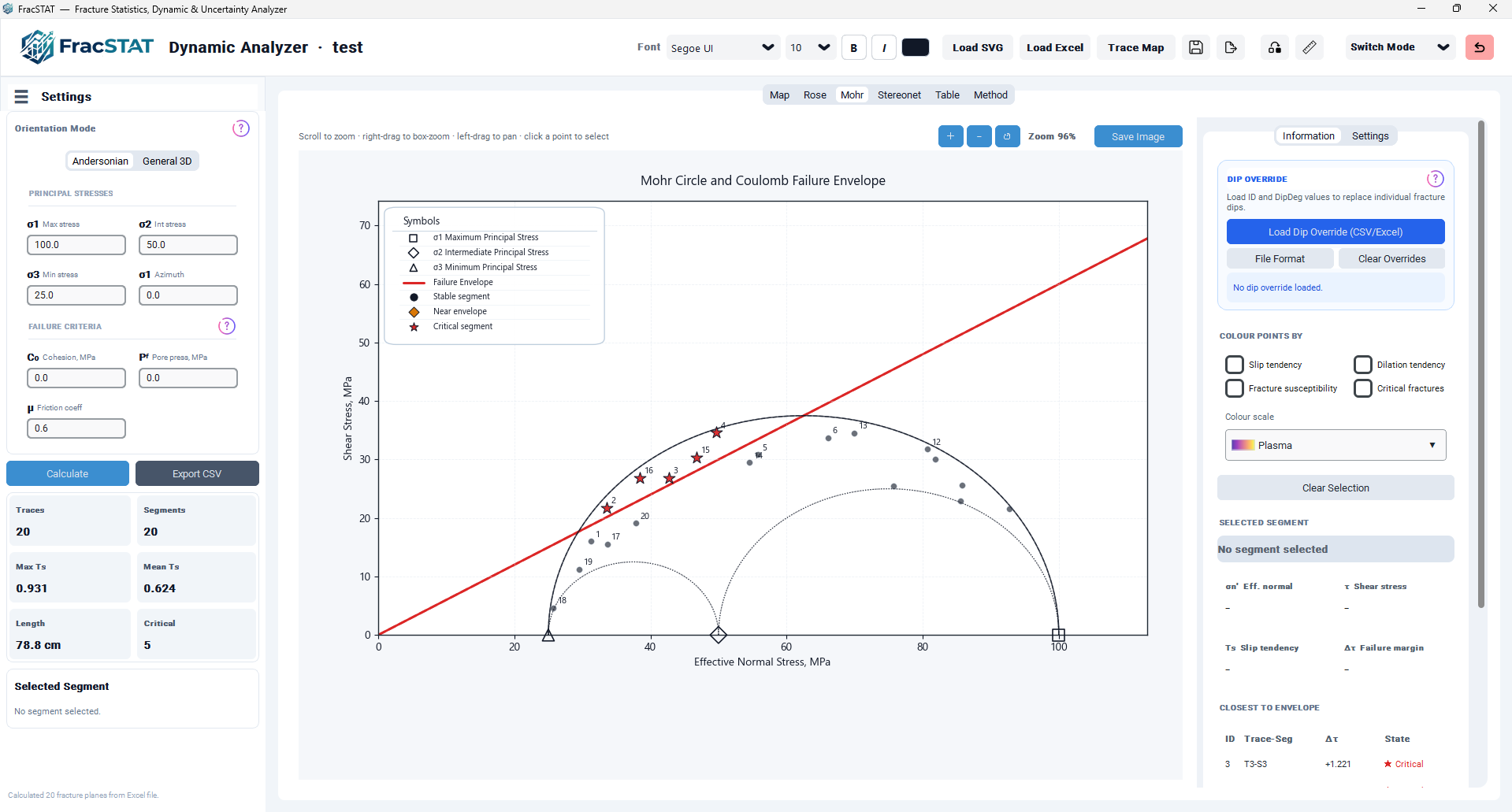
Typical uses of this tab include: rapid triage of which mapped or measured fractures are critically stressed and therefore mechanically active conduits for fluid flow; sensitivity testing of how the failure population changes as pore pressure, cohesion, friction coefficient, or principal stress magnitudes are varied; preparing publication-quality Mohr diagrams with fully customizable colours, symbols, colour bars, and annotation boxes; and cross-referencing individual fractures between the Mohr, Map, Stereonet, and Table views via a shared segment-selection mechanism.
2. Interface Overview
The Mohr Tab is divided into two principal regions: a plotting canvas occupying the majority of
the tab, and a fixed-width scrollable side panel on the right containing two inner tabs,
"Information" and "Settings", implemented as a nested CTkTabview.
2.1 Plot Canvas and Toolbar
A thin toolbar sits above the Matplotlib canvas. From left to right it presents: a hint label describing the available mouse interactions ("Scroll to zoom · right-drag to box-zoom · left-drag to pan · click a point to select"); a Save Image button that exports the current figure at the project's configured export DPI; a compact zoom control group ("+" zoom-in, "−" zoom-out, "↺" reset view); and a live zoom-percentage label. The canvas itself hosts the Mohr circles, the failure envelope, every plotted fracture pole, the principal-stress markers, an optional colour-mapped tendency field, and a draggable "Symbols" legend box.
2.2 Side Panel — Information Tab
The Information tab is the primary working panel for day-to-day interpretation. From top to bottom it contains: the Dip Override card (shared with the Stereonet tab), a "Colour Points By" card offering four mutually exclusive metric checkboxes plus a colour-scale dropdown, a "Clear Selection" button, a coloured "Selected Segment" status badge, four resolved-stress metric tiles for the currently selected fracture, and a "Closest to Envelope" ranking table with a "Show in Map" navigation button.
2.3 Side Panel — Settings Tab
The Settings tab exposes every cosmetic and layout parameter of the diagram, organized into five cards: Pole Styling, Display Options, Plot Elements, Layout & Sizing, and a final Reset Defaults action. These controls do not affect the underlying stress calculation; they govern only how the already-computed results are rendered.
3. Data Input
The Mohr Tab consumes two data structures that are populated elsewhere in the Dynamic Analyzer workspace and simply read (never recomputed) by this tab:
| Attribute | Role |
|---|---|
self.results | The pandas DataFrame returned by core/calculator.py's run_calculation(), containing one row per fracture segment or fracture plane with columns including StrikeDeg, DipDeg, SigmaN, EffectiveSigmaN, Tau, FailureTau, CoulombMargin, EnvelopeDistance, SlipTendency, SlipTendencyNorm, DilationTendency, FractureSusceptibility, FractureSusceptibilityNorm, CriticalStress, CriticalStressValue, CriticalFactor, CriticalState, and CriticalStateValue. |
self.current_stress | A dictionary snapshot of the sidebar's stress inputs at the time "Calculate" was last pressed, holding sigma1, sigma2, sigma3, pore_pressure, cohesion, friction, and (when the General 3D orientation mode is active) sigma1_trend/sigma1_plunge/sigma3_trend. |
Because the Mohr Tab only reads these two objects, no file loading, parsing, or validation occurs
inside this module; all format handling (SVG trace maps, legacy fracture-plane spreadsheets,
Trend/Plunge pole files, and focal-mechanism tables) is the responsibility of
core/svg_loader.py and core/excel_loader.py, and all stress resolution
is the responsibility of core/calculator.py. If self.results is empty
or self.current_stress has not yet been populated (i.e. no successful calculation
has run), the tab renders an empty "Mohr diagram" placeholder title and takes no further action.
3.1 Dip Override Input
A dip-override CSV/Excel file may be loaded from the Information tab's Dip Override card (shared
logic with the Dynamic Analyzer's Map and Stereonet tabs). The file must supply an
ID column matching the segment IDs shown in the Table tab and a
DipDeg column in the range 0–90°. Loading a new file replaces any existing
per-segment dip overrides and immediately triggers recalculation, which updates every Mohr-Tab
pole position the next time the diagram is redrawn.
4. Settings and Controls
This section documents every interactive control in the Mohr Tab, grouped by the card in which
it appears. Unless stated otherwise, every control triggers an immediate redraw of the diagram
(via _draw_mohr, described in Section 7).
4.1 Information Tab — Colour Points By
| Control | Type | Default | Effect |
|---|---|---|---|
| Slip tendency | Checkbox (exclusive) | Unchecked | Colours poles and the background tendency field by SlipTendencyNorm (normalized) or SlipTendency (raw), depending on the "Normalize color scale" checkbox in the Settings Tab's own Display Options (Section 4.5). |
| Dilation tendency | Checkbox (exclusive) | Unchecked | Colours by DilationTendency, always on a fixed 0–1 scale. |
| Fracture susceptibility | Checkbox (exclusive) | Unchecked | Colours by FractureSusceptibility (MPa). |
| Critical fractures | Checkbox (exclusive) | Unchecked | Colours by CriticalStateValue, a four-tier classification (Stable / Near Critical / Critical / Unstable) matching the same bands used by the Rose and Map tabs and by core.calculator.critical_factor_and_state() — see Section 5.3. The colour bar uses a proper colormap/norm with the four state names as tick labels, not a plain two-colour palette. |
| Colour scale dropdown | Custom colour-swatch dropdown | Plasma | Selects the Matplotlib colormap (or the bundled MATLAB-style Parula) applied when any of the four metrics above is active. Ignored when no metric is checked ("no metric" / classic mode, see Section 6.4). |
The four metric checkboxes are mutually exclusive: selecting one automatically clears the others
(change_mohr_metric). Unchecking the active checkbox returns the diagram to "no
metric" / classic mode, in which poles are drawn using the fixed stable/near/critical colour
scheme described in Section 6.4 instead of a continuous colour map.
4.2 Information Tab — Actions and Status
| Control | Type | Effect |
|---|---|---|
| Clear Selection | Button | Deselects the currently highlighted segment across the Mohr, Map, Table, and Stereonet tabs simultaneously (clear_selection). |
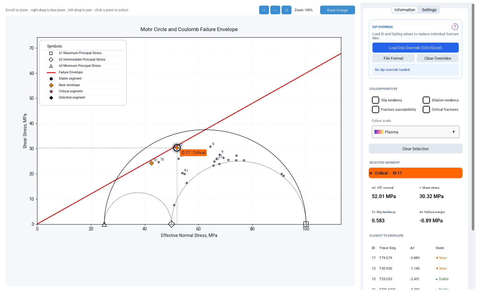
| Selected Segment badge | Status label | Displays "No segment selected" in a neutral colour, or, once a segment is chosen, a star/diamond/circle glyph plus the segment ID with a colour indicating Critical / Near envelope / Stable state. |
| Resolved stress tiles | Four read-only value cards | Show σₙ′ (effective normal stress), τ (shear stress), Tₛ (slip tendency), and Δτ (Coulomb failure margin) for the selected segment. |
| Show in Map | Button | Switches the workspace to the Map tab and centres attention on the currently selected segment (select_segment(..., switch_to_map=True)). |
4.3 Information Tab — Closest to Envelope Table
This eight-row table lists the fractures whose stress state places them nearest to (or past)
the failure envelope, refreshed on every draw by update_mohr_closest_table().
Columns are ID, Trace-Seg (formatted as "T<trace>-S<segment>"), Δτ (signed
Coulomb margin in MPa, positive meaning the point is on or beyond the envelope), and State,
shown as a coloured glyph/word: a red star and "★ Critical" for segments already at or
past failure, an amber diamond and "◆ Near" for segments within 5% of the maximum observed
shear stress of the envelope, and a green circle and "● Stable" otherwise. Rows are
populated from the results sorted by EnvelopeDistance (ascending, i.e. nearest
first); unused rows are blanked with an em-dash.
4.4 Settings Tab — Pole Styling
| Control | Type | Default | Range / Options |
|---|---|---|---|
| Pole shape | Dropdown | Circle | Circle, Diamond, Square, Triangle Up, Star, Cross |
| Pole size | Numeric entry | 48 | Matplotlib scatter marker area, in points² |
| Pole colour | Colour swatch | #FF0000 | Marker face colour when a colour metric is active, and in classic mode via the fixed palette override |
| Pole boundary | Colour swatch | #1F2933 | Marker edge colour |
| Pole boundary width | Numeric entry | 0.45 | Marker edge line width, in points |
4.5 Settings Tab — Display Options
| Control | Type | Default | Effect |
|---|---|---|---|
| Envelope line width | Numeric entry | 2.0 | Line width, in points, of the Mohr–Coulomb failure envelope |
| Custom title | Text entry | (blank → auto) | Overrides the automatic title "Mohr Circle and Coulomb Failure Envelope" (with the active metric name appended when applicable) |
| Mohr envelope without Pore Pressure | Checkbox | Checked | Toggles the dry-envelope overlay described in Section 6.6 (dashed circles/line using σₙ instead of σₙ′) |
| Envelope line in front of Mohr Circle | Checkbox | Off (On after Reset Defaults) | Controls the Matplotlib z-order of the failure-envelope line relative to the shear-stress field / circles, so the line can be forced to always render on top |
Normalize color scale (mohr_normalized_var) | Checkbox | Checked | When a metric-based colouring mode is active, switches between the normalized (SlipTendencyNorm, per-dataset min–max scaled to [0, 1]) and raw (SlipTendency) values used for the colour mapping. Toggling it triggers a preserve_view redraw of both the Mohr Tab and, if present, the Stereonet Tab, so the two stay in sync. |
4.6 Settings Tab — Plot Elements
| Control | Type | Default | Effect |
|---|---|---|---|
| Outer background | Colour swatch | #F5F7FA | Figure (page) background colour |
| Plot background | Colour swatch | #FFFFFF | Axes background colour |
| Grid colour | Colour swatch | #D9E2EC | Colour of the dashed reference grid |
| Envelope shade | Colour swatch | #DC2626 | Reserved accent colour used in the failure-region shading logic |
| Envelope line | Colour swatch | #DC2626 | Line colour of the Mohr–Coulomb envelope (and, tinted, the Symbols index entry for it) |
| Fracture plane | Colour swatch | #FF0000 | Reserved colour for fracture-plane trace overlays |
| Show grid lines | Checkbox | Checked | Toggles the dashed background grid |
| Grid line width | Numeric entry | 0.6 | Width of grid lines, in points |
| Boundary colour | Colour swatch | #1F2933 | Colour of the plot's outer axis spines |
| Boundary width | Numeric entry | 1.0 | Width of the plot's outer axis spines, in points |
4.7 Settings Tab — Layout and Sizing
This card controls the physical pixel dimensions of the rendered figure and the geometry of its colour bar. By default the plot canvas fills whatever space is available in its parent panel ("auto" mode); typing a value into either pixel field switches the canvas into a fixed-size mode.
| Control | Type | Default | Effect |
|---|---|---|---|
| Plot Width (px) | Numeric entry | 1000 | Forces the rendered figure to this pixel width once edited |
| Plot Height (px) | Numeric entry | 800 | Forces the rendered figure to this pixel height once edited |
| Colour bar Length (0.0–1.0) | Numeric entry | 1.0 | Fractional length of the horizontal colour bar relative to the figure width |
| Colour bar Thickness (0.0–1.0) | Numeric entry | 0.025 | Fractional thickness of the colour bar |
| Colour bar Bottom Margin | Numeric entry | 0.09 | Fractional vertical offset of the colour bar from the bottom of the figure |
| Reset to Auto (fill plot area) | Button | — | Clears the fixed-size mode and returns the canvas to filling its parent panel automatically |
4.8 Reset Defaults
The Reset Defaults button at the bottom of the Settings tab restores every colour, width, toggle, and size field listed in Sections 4.4–4.7 to its factory value in a single action and forces two consecutive redraws to guarantee the change is reflected immediately, including the plot returning to automatic (fill-parent) sizing.
5. Mathematical Background
This section defines every quantity plotted or reported by the Mohr Tab. All stress values are expressed in MPa and all angles in degrees unless stated otherwise. σ₁ ≥ σ₂ ≥ σ₃ denote the maximum, intermediate, and minimum principal stresses respectively; P_f is pore pressure; C₀ is cohesion; μ is the coefficient of internal friction. The conventions and derivations follow standard rock-mechanics treatments (Jaeger et al., 2007; Zoback, 2007).
5.1 Mohr Circle Construction
For each principal-stress pair (σᵢ, σᵧ) the corresponding Mohr circle has:
The Mohr Tab draws three such circles: the outer (σ₁–σ₃) circle in a solid line, and the two inner (σ₁–σ₂) and (σ₂–σ₃) circles in a dotted line, each parameterized as:
Because pore pressure acts equally on all faces, the diagram is drawn in effective-stress space by subtracting P_f from every σ coordinate before plotting (the circle centres shift left by P_f, radii are unchanged) — the Terzaghi effective-stress convention that underlies fault-reactivation analysis (Sibson, 1985). This assumes an isotropic, unit Biot coefficient; anisotropic poroelastic response is not modelled (Healy, 2012).
5.2 Effective Normal Stress and Failure Envelope
The envelope is drawn as a straight line from the origin region out to a value far beyond the data range (ten times the maximum σ plus a fixed margin), so that it never appears to terminate abruptly inside the visible axes regardless of zoom level; only the visible portion is used when auto-scaling the y-axis.
5.3 Coulomb Failure Margin and Critical Stress
A segment is flagged CriticalStress = True when Δτ ≥ 0, i.e. the
resolved shear stress equals or exceeds the frictional strength available at that effective
normal stress — the fracture is predicted to be at or past the point of frictional sliding
under the entered stress state. EnvelopeDistance is defined as |Δτ|, used
purely for ranking proximity to the envelope irrespective of sign.
The "Near envelope" classification used for the badge and the closest-to-envelope table applies
when a non-critical segment's EnvelopeDistance is within 5% of the maximum τ
observed across the whole dataset, i.e. EnvelopeDistance ≤ 0.05 ×
max(τ). This is a relative, dataset-dependent threshold rather than a fixed MPa tolerance,
so its meaning should be re-checked whenever the stress magnitudes change substantially.
A separate, four-tier classification is also computed for every segment via
core.calculator.critical_factor_and_state(): CriticalFactor is the
friction coefficient required to resist the resolved shear stress,
(τ − C0) / (σn′), and threshold_ratio expresses that demand
as a fraction of the entered friction coefficient μ. The resulting CriticalState
/ CriticalStateValue bands this ratio into Stable (0–50%), Near Critical
(50–75%), Critical (75–100%), or Unstable (>100%). Unlike the binary
CriticalStress flag above, this is not tied to the specific τ ≥ C0 +
μ·σn′ envelope test; it instead measures how close each fracture's
friction demand is to the failure threshold, and is the classification driving the Mohr Tab's
"Critical fractures" colour metric (Section 4.1) as well as the equivalent
metric in the Rose and Map tabs.
5.4 Tendency and Susceptibility Metrics
These are computed upstream in core/calculator.py and simply displayed here. Slip
tendency and its normalization follow
Morris et al. (1996), dilation tendency follows
Ferrill and Morris (2003), and fracture
susceptibility — the pore-pressure increase required to bring a plane to failure —
follows Streit and Hillis (2004):
Ts,max is the theoretical maximum τ/σn achievable over every possible fracture orientation for the given stress tensor — a closed-form function of σ₁ and σ₃ only, equal to the tangent from the origin to the outer Mohr circle — not the maximum among only the loaded fractures. Dilation tendency ranges 0 (least likely to dilate/open) to 1 (most likely). Fracture susceptibility is expressed directly in MPa and is not bounded to [0, 1]; when the "normalized" display option is active, the Mohr Tab rescales it per-dataset from the loaded fractures' observed Sf minimum and maximum and then inverts the result, Sf,norm = 1 − (Sf − min) / (max − min), so that the lowest Sf — the smallest remaining pore-pressure margin, i.e. the plane closest to failure — maps to 1.0 at the "hot" end of the colormap. Without that inversion the colour scale reads backwards, rendering stable planes as critical. Because the endpoints come from the loaded data rather than from theory, Sf,norm = 1.0 means "least stable plane in this file", not "at failure", and should not be compared across datasets; if every segment shares one Sf value (range below 10⁻¹²) the field is set to 0 throughout instead of dividing by zero.
calculator.py actually computes two Sf values side by side, one
per historical version of the reference MATLAB script: FractureSusceptibility is
the updated formula shown above (pore pressure and cohesion corrected), while
FractureSusceptibilityLegacy reproduces the original script's σn −
τ/μ, with no pore-pressure or cohesion term. The two differ by exactly the pore
pressure Pf when cohesion is zero. The Mohr Tab's colour-by and background-field options use only
the updated FractureSusceptibility value; the legacy value is carried through for
cross-checking against older MATLAB output and is surfaced in the Table tab
as its own column so both figures are available without re-running the calculation.
5.5 Continuous Tendency Field Over All Orientations
In addition to plotting the discrete poles of the loaded fractures, the Mohr Tab shades the background of the diagram with a continuous field showing what the active tendency metric would be for a fracture of any possible orientation subjected to the same stress tensor. The field is evaluated on a dense polar/azimuthal mesh of unit-normal directions:
with φ spanning a 58-point grid over (0.01, π/2 − 0.01) and θ spanning a 116-point grid over [0, 2π). For every (φ, θ) pair the appropriate colour metric — normalized slip tendency, dilation tendency, fracture susceptibility, or the binary critical-stress indicator — is evaluated using the same formulas as Section 5.4, each point is mapped into (σn′, τ) space, and the resulting scattered points are triangulated and filled with a 28-level contour plot (Section 6.5).
6. Algorithms
6.1 Field Sampling and Triangulation Masking
The (σn′, τ) points generated by the polar mesh of Section 5.5 are triangulated
with Matplotlib's Delaunay-based Triangulation. Because the physically meaningful
region of the Mohr plane lies only within the area bounded by the outer Mohr circle and outside
the two inner circles, every triangle whose centroid falls inside either the
(σ₂–σ₃) or (σ₁–σ₂) inner circle is
masked out of the triangulation before contouring, keeping the shaded region visually consistent
with the classical three-circle Mohr diagram.
6.2 Envelope Extension and Auto-Scaling
To avoid the visual artefact of the failure-envelope line stopping abruptly within the visible plot area, the envelope is sampled over a domain extending to 10× the maximum σ value plus a 500 MPa margin. The vertical (y) axis limit is then computed only from the portion of that line that actually falls within the horizontal view window, so that the automatic y-scaling responds sensibly to zoom rather than being dominated by the artificially extended tail of the envelope line.
6.3 Selected-Segment Reticle
When a segment is selected (by clicking a point, a Table row, or a Stereonet pole), the Mohr Tab draws a dotted horizontal/vertical crosshair from the axes edges to the point, followed by two concentric open circles (a faint wide halo and a crisp inner ring) and a plus-shaped marker at the exact coordinate, plus a rounded annotation box reading "ID <n>" anchored with a small offset so it does not obscure the point itself.
6.4 Classic (No-Metric) Colour Mode
When none of the four colour-metric checkboxes is active, poles are drawn in three fixed groups rather than on a continuous colour scale, each with its own marker shape, size, and transparency for maximum discriminability at a glance:
| Group | Marker | Colour | Condition |
|---|---|---|---|
| Stable | Circle ('o'), small, semi-transparent | Muted grey/theme colour | Not critical and EnvelopeDistance > 5% of max τ |
| Near envelope | Diamond ('D'), medium | Amber / "effective" accent | Not critical and EnvelopeDistance ≤ 5% of max τ |
| Critical | Star ('*'), largest | Red / "failure" accent | CriticalStress == True |
Each of these three scatter collections is registered as a separate matplotlib "pick" artist so that mouse clicks correctly resolve to the underlying segment ID regardless of which group the point belongs to. In this mode the top 20 critical points (by descending Coulomb margin) and the 10 non-critical points closest to the envelope are also labelled directly on the plot with their integer segment ID.
6.5 Metric-Driven Colour Mode
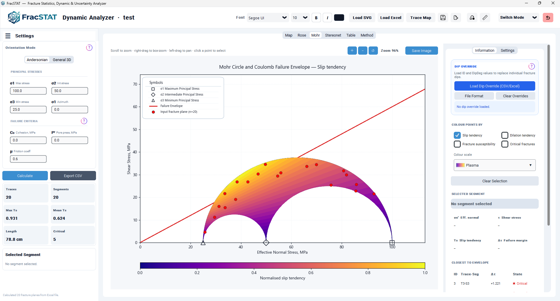
When a metric checkbox is active, the workflow is: (1) build the continuous background field as
in Section 5.5 and render it with tricontourf at 28 levels using the selected
colormap and a Normalize (or, for the Critical fractures metric, the four-tier
colormap/norm returned by attribute_colormap_and_norm(), matching the discrete
Stable/Near Critical/Critical/Unstable bands described in Section 5.3); (2) scatter every loaded fracture's (σn′, τ) point on top using the
user-configured pole shape, size, colour, and edge styling; (3) attach a horizontal colour bar
sized and positioned per the Layout & Sizing settings (Section 4.7), labelled with the
metric's descriptive name and, for the Critical fractures metric, custom tick labels "Stable" /
"Near Critical" / "Critical" / "Unstable" instead of numeric ticks.
@staticmethod
def _mohr_field(sigma1, sigma2, sigma3, pore_pressure, cohesion, friction, value_column, df=None):
    polar   = np.linspace(0.01, np.pi / 2 - 0.01, 58)
    azimuth = np.linspace(0.0, 2 * np.pi, 116, endpoint=False)
    polar, azimuth = np.meshgrid(polar, azimuth)
    n1 = np.sin(polar) * np.cos(azimuth)
    n2 = np.sin(polar) * np.sin(azimuth)
    n3 = np.cos(polar)
    sigma_n     = sigma1 * n1**2 + sigma2 * n2**2 + sigma3 * n3**2
    traction_sq = sigma1**2 * n1**2 + sigma2**2 * n2**2 + sigma3**2 * n3**2
    tau         = np.sqrt(np.maximum(traction_sq - sigma_n**2, 0.0))

    if value_column.startswith("SlipTendency"):
        raw = tau / np.maximum(sigma_n, 1e-12)
        if value_column == "SlipTendencyNorm":
            # Exact closed-form theoretical max, as in calculator.py --
            # NOT raw.max() over this mesh.
            denom = 2.0 * np.sqrt(max(sigma1 * sigma3, 1e-12))
            tsmax = max((sigma1 - sigma3) / denom, 1e-12)
            values = raw / tsmax
        else:
            values = raw
    elif value_column == "DilationTendency":
        values = (sigma1 - sigma_n) / max(sigma1 - sigma3, 1e-12)
    elif value_column.startswith("FractureSusceptibility"):
        raw_values = sigma_n - pore_pressure - (tau - cohesion) / max(friction, 1e-12)
        if value_column == "FractureSusceptibilityNorm" and df is not None and not df.empty:
            # Inverted: a SMALLER Sf is MORE susceptible, so it maps to 1.0.
            sf_min = float(df["FractureSusceptibility"].min())
            sf_max = float(df["FractureSusceptibility"].max())
            sf_range = sf_max - sf_min
            values = (np.zeros_like(raw_values) if abs(sf_range) < 1e-12
                      else 1.0 - (raw_values - sf_min) / sf_range)
        else:
            values = raw_values
    else:
        values = (tau >= cohesion + friction * (sigma_n - pore_pressure)).astype(float)
    return sigma_n.ravel() - pore_pressure, tau.ravel(), values.ravel()
The _mohr_field() helper, evaluating slip tendency, dilation tendency, fracture susceptibility, or critical fracture state over the full polar/azimuthal mesh of possible plane orientations.
6.6 Dry-Envelope Overlay
When "Mohr envelope without Pore Pressure" is enabled, a second, independent overlay is drawn on the same axes using raw (non-effective) stresses: the three Mohr circles are redrawn in a muted, dashed style, and a dashed failure line τ = μ·σ (i.e. with cohesion and pore pressure both omitted) is added. This lets the analyst directly compare how much pore-pressure reduction shifts the failure envelope and the data cloud relative to the theoretical dry (undrained-free) case, without needing to re-run the calculation with P_f = 0.
_draw_mohr_dry_overlay() respects the caller's preserve_view flag when
expanding the x-axis limits to fit the dry envelope line: the expansion is skipped entirely when
preserve_view is true. Previously this expansion ran unconditionally, so any
cosmetic-only redraw with the dry overlay enabled would silently reset the user's pan/zoom
viewport back out to fit the full envelope. It is now applied only on non-preserve_view
redraws, consistent with the axis-limit handling in the rest of _draw_mohr
(Section 7).
6.7 Symbols Index Construction
The floating "Symbols" legend box is built entirely from primitive Matplotlib artists (a rounded
FancyBboxPatch, text labels, marker scatters, and thin separator lines) rather than
Matplotlib's built-in Legend class, so that its position, size, and content can be fully
controlled and made draggable. Its rows always include the three principal-stress markers
(σ₁ square, σ₂ diamond, σ₃ triangle) and the
failure-envelope line swatch; when no metric is active it additionally lists the three classic
pole states (Stable / Near / Critical), and when a metric is active it instead lists a single
"Input fracture plane (n=<count>)" row using the user's chosen pole shape and colours. A
"Selected segment" row is appended whenever a segment is currently selected. The box's width is
computed from the longest label string and the height from the row count, both scaled by the
ratio of the current global font size to a 10-pt baseline, so the legend remains legible and
proportionate when the workspace font size is changed in the header.
6.8 Hover Tooltip / Nearest-Point Lookup
On mouse movement over the axes (when not currently panning, box-zooming, or dragging the Symbols index), the Mohr Tab computes the axes-fraction distance from the cursor to every plotted (σn′, τ) point simultaneously (vectorized with NumPy, normalized independently by the current x- and y-axis spans so the test is not distorted by non-square aspect ratios), and if the nearest point lies within a small fractional threshold (0.02) it displays a floating annotation with that segment's ID, trace/segment numbers, σn′, and τ. The same annotation object is reused and repositioned/re-labelled on subsequent moves rather than being recreated, avoiding flicker and unnecessary allocation.
7. Internal Workflow
The complete redraw pipeline, _draw_mohr(preserve_view=False), executes the
following ordered steps every time any control in this tab changes, a segment is
selected/cleared, or the tab receives fresh calculation results:
- Apply the current canvas sizing mode (auto-fill vs. fixed pixel dimensions) via
_mohr_apply_canvas_sizing(). - Read and numerically validate every Settings-tab field (grid width, envelope width, boundary width, pole size/width, colour-bar geometry), silently falling back to a sensible default for any field that cannot be parsed as a float.
- Preserve the current axis limits if
preserve_viewis requested (used for cosmetic-only redraws so the user's pan/zoom state is not lost). - Clear the axes, the colour-bar axes, and any cached pick/hover/drag state.
- If
self.resultsis empty orself.current_stresshas not been populated, render the placeholder title and return early. - Draw the three Mohr circles in effective-stress space (Section 5.1).
- Classify every segment as critical / near / stable using the Section 5.3 thresholds.
- Branch on whether a colour metric is active: draw either the three fixed-style scatter groups (Section 6.4) or the continuous field plus single scatter layer and colour bar (Section 6.5).
- Compute axis extents, including the extended envelope line and its visible-window-only vertical scaling (Section 6.2).
- Draw the selected-segment reticle, if any (Section 6.3).
- Draw the failure-envelope line at the z-order implied by "Envelope line in front of Mohr Circle".
- Draw the three principal-stress markers.
- In classic mode only, label the most significant critical/near points with their segment IDs.
- Refresh the Closest-to-Envelope table (Section 4.3).
- Set the plot title (custom or automatic), axis labels, grid, and spine styling.
- Cache the arguments used to build the Symbols index and draw it (Section 6.7).
- Apply either the preserved axis limits or the freshly computed home limits.
- Update the on-screen zoom percentage label.
- If the dry-envelope overlay is enabled, draw it on top (Section 6.6).
- Request a canvas redraw (
draw_idle).
7.1 Segment Selection Propagation
Selecting a fracture (by clicking a pole in the Mohr Tab, a row in the Table tab, or a pole in
the Stereonet tab) calls the shared SlipTendencyApp.select_segment() method, which
updates the sidebar's "Selected Segment" free-text summary, calls
update_mohr_selection_panel() to refresh the four resolved-stress metric tiles,
updates the coloured status badge, and triggers a preserve_view redraw of the Mohr,
Map, and Stereonet tabs so the same fracture is highlighted consistently everywhere in the
workspace.
8. Statistical Methods
The Mohr Tab performs lightweight descriptive/ranking statistics rather than inferential statistics; the quantitative modelling (Monte Carlo, distribution fitting, etc.) lives in the separate Uncertainty Analyzer module. The statistics implemented directly in this tab are:
| Statistic | Definition | Purpose |
|---|---|---|
| max(τ) | Maximum shear stress across all loaded segments | Establishes the relative 5% "near envelope" threshold |
| EnvelopeDistance ranking | |Δτ| sorted ascending | Produces the 8-row Closest to Envelope table and the classic-mode point-labelling priority list |
| Coulomb margin ranking (critical subset) | Δτ sorted descending, top 20 | Prioritizes which critical points receive an on-plot ID label so the busiest region of the diagram remains legible |
| Field normalization | Per-metric min–max or fixed 0–1 scaling, or 2-class boundary for the binary metric | Ensures the colour bar and colour-mapped points are on a consistent, metric-appropriate scale each time the metric or data changes |
9. Visualization
9.1 Plot Anatomy
A single Matplotlib Axes hosts the entire diagram: x-axis "Effective Normal Stress, MPa", y-axis "Shear Stress, MPa". Overlaid elements, from back to front by default, are: the coloured tendency field (metric mode only) or nothing (classic mode); the three Mohr circles; the failure envelope (z-order configurable); the dry-envelope overlay (if enabled); the scatter layer(s) of fracture poles; the principal-stress markers; the selected-segment reticle; point ID labels (classic mode); and the floating Symbols index box.
9.2 Colour Bar Geometry
The colour bar is a dedicated secondary Axes (mohr_cbar_ax) whose rectangle [left,
bottom, width, height] in figure-fraction coordinates is recomputed on every draw from the
Layout & Sizing length/thickness/bottom-margin fields, automatically centred horizontally as
(1 − length)/2. If any of the three fields cannot be parsed as a float, the colour bar
falls back to a fixed default rectangle.
9.3 Save Image
The toolbar's "Save Image" button calls the shared SlipTendencyApp.save_plot_image()
routine, which writes the current figure to
<project>/FracSTAT_plot_exports/<project name>/ as a PNG named from the
project, tab, active metric, colour scale, and a timestamp, at the DPI configured in Settings
→ Export DPI (default 300). The figure is saved with a tight bounding box so that
out-of-axes elements such as the Symbols index box are not clipped.
10. Advanced Features
10.1 Pan, Zoom, and Box-Zoom
| Interaction | Trigger | Behaviour |
|---|---|---|
| Scroll wheel | Mouse wheel over the axes | Zooms in/out centred on the cursor position by a factor of 0.85 (in) / 1.18 (out) per notch |
| Left-drag | Hold left mouse button and move | Pans the view by translating both axis limits by the dragged data-space delta |
| Right-drag | Hold right mouse button and move | Draws a dashed rubber-band rectangle; releasing zooms the view to exactly that rectangle |
| + / − toolbar buttons | Click | Zoom in (0.72×) / out (1.35×) centred on the current view centre |
| ↺ Reset view | Click | Restores the axis limits captured as "home" on the most recent full redraw |
10.2 Move Elements Mode and Draggable Symbols Index
When the workspace-wide "Move Elements" toggle (in the shared header) is active, a left-click
that lands inside the Symbols index box's current footprint begins a drag operation instead of a
pan. Mouse motion updates the box's anchor position in axes-fraction coordinates (clamped to a
generous but finite range so it cannot be dragged indefinitely off-screen), and only the index
artists are removed and rebuilt on each motion event
(_redraw_mohr_symbol_index) rather than re-running the full
_draw_mohr() pipeline, keeping the drag interaction smooth even on larger datasets.
The chosen position persists across subsequent redraws.
10.3 Manual Plot Pixel Sizing
By default the Mohr canvas is gridded with sticky="nsew" so it automatically fills
its parent panel and resizes smoothly with the application window. The first time the user
commits a value into the Plot Width or Plot Height fields (via Enter or focus-out), the tab
switches into a fixed-pixel-size mode: the Matplotlib Figure's internal resolution is set from
the requested width/height in pixels divided by its DPI, and the underlying Qt widget is
re-gridded without the sticky option so the grid geometry manager can no longer stretch it. This
avoids a documented race condition in which sticky="nsew" and an explicit
widget.configure(width=..., height=...) call would compete on every window resize,
occasionally leaving a stale or partially redrawn frame visible underneath the new one. "Reset
to Auto" reverses this by re-enabling sticky-fill behaviour.
10.4 Cross-Tab Selection Synchronization
Because segment selection state (self.selected_segment_id) is owned by the parent
SlipTendencyApp rather than by any individual tab, clicking a pole here, a row in
the Table tab, or a pole in the Stereonet tab all converge on the same
select_segment() call, guaranteeing that the reticle in the Mohr Tab, the
highlighted row in the Table tab, the halo marker in the Map tab, and the highlighted pole in
the Stereonet tab always agree on which single fracture is currently of interest.
11. Performance Optimization
| Technique | Where Applied | Benefit |
|---|---|---|
Cached Symbols-index arguments (_mohr_index_last_args) | Drag interaction for the Symbols box | Lets a mouse-drag redraw only the small legend box instead of the entire diagram on every motion event |
| Vectorized nearest-point search | Hover tooltip | Uses NumPy array operations across all points simultaneously instead of a Python-level loop, keeping hover responsive even for large datasets |
| Auto vs. fixed canvas sizing with conditional sticky grid option | _mohr_apply_canvas_sizing() | Prevents a documented Matplotlib canvas resize race condition that could otherwise cause visible frame corruption on window resize |
| Separate pick-artist registries per scatter group | Classic mode click handling | Allows constant-time identification of which segment was clicked, regardless of which of the three stable/near/critical groups it belongs to |
| Numeric field parsing with fallback defaults | Every Settings-tab entry | Avoids exceptions (and therefore a broken redraw) if the user temporarily leaves a field blank or enters non-numeric text while editing |
| Bounded 58×116 polar grid | Continuous tendency field | Balances visual smoothness of the background contour against the cost of re-evaluating stress equations and re-triangulating on every redraw |
12. Practical Examples
Example 12.1 — Identifying Critically Stressed Fractures for Reservoir Stimulation
- Load an SVG trace map or Excel orientation table of fractures via the workspace header, then enter the site's principal stresses, pore pressure, cohesion, and friction coefficient in the sidebar and press Calculate.
- Open the Mohr Tab and check the "Critical fractures" colour-metric checkbox to shade the diagram by the four-tier Stable/Near Critical/Critical/Unstable field.
- Inspect the Closest to Envelope table to identify the specific fracture IDs already at or nearest to failure.
- Click one of the listed critical fractures to inspect its resolved σn′, τ, Tₛ, and Δτ in the metric tiles, then use "Show in Map" to see its spatial location.
- Re-run the calculation with a higher assumed pore pressure (e.g. simulating fluid injection) to observe how many additional fractures cross into the critical population, using the dry-envelope overlay to compare against the undrained case.
Example 12.2 — Preparing a Publication-Quality Mohr Diagram
- Select the desired colour metric (e.g. Fracture susceptibility) and colour scale (e.g. Viridis) in the Information tab.
- In the Settings tab, set the pole shape to Diamond, increase Pole size for visibility, and choose complementary Outer/Plot background colours.
- Enter a custom title describing the study area and stress case.
- Under Layout & Sizing, set an explicit Plot Width/Height (e.g. 1600×1200 px) suitable for the target publication figure size, and adjust colour-bar length/thickness accordingly.
- Enable Move Elements mode from the header to reposition the Symbols index box clear of the data cloud, then click Save Image to export a 300 DPI PNG.
13. Geological Interpretation
The Mohr–Coulomb construction visualized in this tab is the standard framework used in structural geology and reservoir geomechanics to assess the frictional stability of pre-existing planes of weakness — joints, faults, or bedding-parallel fractures — under a given in-situ stress state.
- Points plotting on or above the failure envelope (
CriticalStress = True, Δτ ≥ 0) represent fractures predicted to be frictionally unstable: the resolved shear stress equals or exceeds the frictional resistance available at that effective normal stress. In the field, such orientations are the ones most likely to have accommodated recent slip, to host fluid flow along dilated segments, or to be reactivated by an increase in pore pressure (e.g. injection-induced seismicity) (Sibson, 1985). - Points plotting well below and to the right of the envelope, at high effective normal stress and low shear stress, represent fractures oriented close to a principal stress direction; these are mechanically stable and, absent significant pore-pressure increase, unlikely to slip.
- Slip tendency (Ts) provides a continuous, normalized analogue of the same idea and is often mapped in colour across a fracture network to highlight which structural trends are, as a population, closest to reactivation — useful for ranking candidate flow pathways even where an explicit cohesion/friction pair is uncertain (Morris et al., 1996; Worum et al., 2004).
- Dilation tendency (Td) highlights fractures oriented such that the normal stress acting across them is minimized relative to σ₁; such fractures are mechanically favoured to open (dilate) rather than to shear, and are frequently associated with enhanced permeability in fractured reservoirs even when they are not necessarily close to shear failure (Ferrill and Morris, 2003).
- Fracture susceptibility (Sf) combines the effective normal stress and shear/cohesion/friction terms into a single MPa-valued index used in some legacy fracture-stability workflows; lower (more negative) values indicate a fracture closer to, or already past, the failure criterion. Read as a pore-pressure margin, it is the quantity used to set sustainable injection pressures (Streit and Hillis, 2004).
Because the whole analysis is Andersonian or general 3D depending on the sidebar's Orientation Mode, the geological validity of the Mohr diagram is tied directly to how well the entered principal-stress magnitudes and orientations represent the true in-situ stress tensor at the site; users should treat outputs as conditional on that stress model and re-run sensitivity cases (Section 12.1) wherever the stress tensor is poorly constrained.
14. Implementation Notes
The Mohr Tab is implemented as the MohrTab mixin class in
dynamic_analyzer/tabs/dynamic_mohr_tab.py, mixed into SlipTendencyApp
alongside MapTab, RoseTab, TableTab,
MethodTab, and StereonetTab. It shares several cross-cutting
facilities with its sibling tabs rather than re-implementing them:
| Shared facility | Also used by |
|---|---|
_active_mohr_metric() / change_mohr_metric() | Consulted by the Stereonet tab so both diagrams always agree on the selected stress-tendency metric. |
colormap_from_name(), _attribute_norm(), _colour_scale_definitions() | Provided by SlipTendencyApp itself and shared by the Map, Rose, Mohr, and Stereonet tabs, ensuring a single consistent set of named colour scales across the whole workspace. |
_build_dip_override_card() | A shared sidebar-construction helper also used by the Stereonet tab, so the two tabs' Dip Override cards stay visually and behaviourally identical. |
plot_palette() | Supplies theme-aware default colours (text, muted, spine, failure, effective) that several Settings-tab defaults are seeded from when the workspace theme changes. |
All colour and dimension fields are backed by ui_common.qtk StringVar/BooleanVar instances
lazily initialized in _mohr_init_vars(), which only creates a variable if it does
not already exist — this makes the initialization function safe to call repeatedly (e.g.
across a project session restore) without discarding values the user has already set.
core/calculator.py computes fracture susceptibility twice per run —
FractureSusceptibility (pore-pressure and cohesion corrected) and
FractureSusceptibilityLegacy (the original, uncorrected MATLAB formula) — so
that results can be cross-checked against either version of the reference script without
re-running the calculation (see Section 5.4). Only the corrected column feeds
the Mohr Tab's own displays; both columns are populated in self.results and are
available to the Table tab.
15. Limitations
| Limitation | Description |
|---|---|
| Bounded background field resolution | The continuous background tendency field is sampled on a fixed 58×116 polar/azimuthal grid; it is a smooth visual guide to the full orientation space rather than an exhaustive enumeration, and very thin features of the failure surface could in principle be under-resolved at that grid density. |
| Coupled pixel size and DPI | Manual pixel sizing fixes the on-screen and exported figure resolution together; changing DPI in the application Settings page after fixing a pixel size changes the physical (inches) size of the exported PNG. |
| Linear Coulomb envelope only | Failure is modelled by a single straight line τ = C₀ + μ·σn′. No curved, pressure-dependent, or bi-linear envelope is offered, and no tensile cut-off is applied at negative σn′, so predictions at very low or negative effective normal stress should be treated with caution (Jaeger et al., 2007). |
| Friction and cohesion are user constants | μ and C₀ are single values applied to every fracture. Real friction coefficients vary with lithology, roughness, mineral coating, and normal stress; laboratory values cluster near μ ≈ 0.6–0.85 but are not universal (Byerlee, 1978). No per-fracture or per-set assignment is supported. |
| Stress tensor is uniform and user-supplied | One homogeneous stress tensor is applied across the whole dataset, entered by hand rather than inverted from data. Results are entirely conditional on that stress model and carry no uncertainty; constraining an in-situ tensor requires independent borehole or focal-mechanism data (Zoback, 2007). |
| Isotropic effective stress | Pore pressure is subtracted directly from each normal stress, i.e. a Biot coefficient of unity and isotropic poroelastic response. Anisotropic or fracture-compliance-dependent responses to pore-pressure change are not represented (Healy, 2012). |
| Dataset-relative normalization | Normalized fracture susceptibility is rescaled from the loaded file's own minimum and maximum (Section 5.4), so Sf,norm = 1.0 means "least stable plane in this file", not "at failure". Values must not be compared between datasets, and the same caution applies to the relative 5% "near envelope" threshold, which also scales with max(τ) in the loaded data. |
| Static, single-realisation analysis | The tab evaluates one stress state at one instant. It does not model slip-induced stress redistribution, fault interaction, time-dependent healing, or the progressive reactivation sequence that numerical slip-tendency studies address (Worum et al., 2004); sensitivity to the stress model must be explored by re-running cases manually (Section 12.1). |
16. References
Sources are listed alphabetically within each group. In-text citations throughout this page link to the corresponding entry below.
16.1 Rock Mechanics and the Mohr–Coulomb Criterion
- Byerlee, J. (1978). Friction of rocks. Pure and Applied Geophysics, 116(4–5), 615–626. https://doi.org/10.1007/BF00876528
- Jaeger, J. C., Cook, N. G. W., & Zimmerman, R. W. (2007). Fundamentals of Rock Mechanics (4th ed.). Blackwell Publishing, Oxford. ISBN 978-0-632-05759-7.
- Sibson, R. H. (1985). A note on fault reactivation. Journal of Structural Geology, 7(6), 751–754. https://doi.org/10.1016/0191-8141(85)90150-6
- Zoback, M. D. (2007). Reservoir Geomechanics. Cambridge University Press. https://doi.org/10.1017/CBO9780511586477
16.2 Slip, Dilation and Susceptibility Analysis
- Ferrill, D. A., & Morris, A. P. (2003). Dilational normal faults. Journal of Structural Geology, 25(2), 183–196. https://doi.org/10.1016/S0191-8141(02)00029-9
- Healy, D. (2012). Anisotropic poroelasticity and the response of faulted rock to changes in pore-fluid pressure. Geological Society, London, Special Publications, 367(1), 201–214. https://doi.org/10.1144/SP367.14
- Morris, A., Ferrill, D. A., & Henderson, D. B. (1996). Slip-tendency analysis and fault reactivation. Geology, 24(3), 275–278. https://doi.org/10.1130/0091-7613(1996)024<0275:STAAFR>2.3.CO;2
- Streit, J. E., & Hillis, R. R. (2004). Estimating fault stability and sustainable fluid pressures for underground storage of CO₂ in porous rock. Energy, 29(9–10), 1445–1456. https://doi.org/10.1016/j.energy.2004.03.078
- Worum, G., van Wees, J.-D., Bada, G., van Balen, R. T., Cloetingh, S., & Pagnier, H. (2004). Slip tendency analysis as a tool to constrain fault reactivation: A numerical approach applied to three-dimensional fault models in the Roer Valley rift system (southeast Netherlands). Journal of Geophysical Research: Solid Earth, 109(B2), B02401. https://doi.org/10.1029/2003JB002586
16.3 Software
- Harris, C. R., Millman, K. J., van der Walt, S. J., Gommers, R., Virtanen, P., Cournapeau, D., … Oliphant, T. E. (2020). Array programming with NumPy. Nature, 585(7825), 357–362. https://doi.org/10.1038/s41586-020-2649-2
- Hunter, J. D. (2007). Matplotlib: A 2D graphics environment. Computing in Science & Engineering, 9(3), 90–95. https://doi.org/10.1109/MCSE.2007.55
Methods statement for the Mohr Tab. If a figure produced by this tab appears in a publication, the details below are what a reader needs in order to reproduce it, and are what the citations above assume:
Three-circle Mohr diagram in effective-stress space for σ₁/σ₂/σ₃ = … MPa and pore pressure P_f = … MPa, with a linear Coulomb envelope τ = C₀ + μ·σn′ for cohesion C₀ = … MPa and friction coefficient μ = … (Jaeger et al., 2007). Fracture poles coloured by normalized slip tendency (Morris et al., 1996), dilation tendency (Ferrill and Morris, 2003), fracture susceptibility (Streit and Hillis, 2004), or the four-tier critical-state classification of Section 5.3, over a continuous background field evaluated on a 58×116 orientation mesh (Section 5.5). Implemented in NumPy (Harris et al., 2020) and rendered with Matplotlib (Hunter, 2007). Report the full stress tensor, P_f, C₀, μ, the orientation mode (Andersonian or general 3D), and which susceptibility column was used; state that normalized susceptibility is rescaled per dataset and is therefore not comparable between files (Section 5.4).