Dynamic Stereonet Tab
Located at dynamic_analyzer/tabs/dynamic_stereonet_tab.py, the
Stereonet Tab (implemented as the mixin class StereonetTab) is
one of six coordinated views inside the Dynamic Analyzer workspace (the others being Map,
Rose, Mohr, Table, and Method). It renders a lower-hemisphere, equal-area (Schmidt) projection
of every fracture plane currently loaded into the workspace, plotted as poles (points
representing the plane normal). Superimposed on the same projection is a continuous colour
field showing how a chosen stress-derived attribute — slip tendency, dilation tendency,
fracture susceptibility, or a four-tier critical-fracture-state classification — would vary across every
conceivable plane orientation for the stress tensor currently defined in the sidebar. The
combination of discrete, data-derived poles and a continuous theoretical field is what makes
the Stereonet Tab a genuinely predictive tool rather than a simple plotting utility: it lets
the analyst see at a glance whether the orientations actually present in the fractured rock
mass coincide with the orientations that the applied or inferred stress field would drive
toward failure.
Within the broader FracSTAT architecture, the Stereonet Tab consumes the same
self.results DataFrame that feeds the Map, Rose, Mohr, and Table tabs, and it
shares the same stress-resolution outputs (SlipTendencyNorm,
DilationTendency, FractureSusceptibility,
CriticalStateValue) produced by calculator.run_calculation(). It
therefore requires no independent data entry: any SVG trace map or Excel/CSV orientation
table already loaded for the Map tab is automatically available here. The module's scope is
strictly the stereographic (angular) domain — it does not compute spatial statistics (that is
the Rose tab's role) or the Mohr–Coulomb failure-envelope diagram (the Mohr tab's role); rather,
it is the 3-D orientation counterpart to the 2-D Mohr diagram, showing where in orientation
space the fractures sit relative to the full field of possible responses.
Position within FracSTAT
- Static Analyzer — Stereonet Plot tab: purely geometric (strike/dip only), no stress resolution.
- Dynamic Analyzer — Stereonet Tab (this module): stress-informed, colour-coded by the active tendency attribute.
- Dynamic Analyzer — Mohr Tab: the 2-D shear/normal-stress analogue of this 3-D orientation view; both tabs share the same four colour-by metrics and the same selection state.
- Dynamic Analyzer — Map Tab: spatial view of the same segments; clicking a pole here highlights the same segment on the Map.
On this page
- 1. Interface Overview
- 2. Data Input and Preprocessing
- 3. Mathematical Background
- 4. Algorithms
- 5. Settings and Controls
- 6. Internal Workflow
- 7. Statistical Methods
- 8. Visualization Components
- 9. Advanced Features
- 10. Performance Optimization
- 11. Practical Examples
- 12. Geological Interpretation
- 13. Implementation Notes
- 14. Limitations
- 15. References
1. Interface Overview
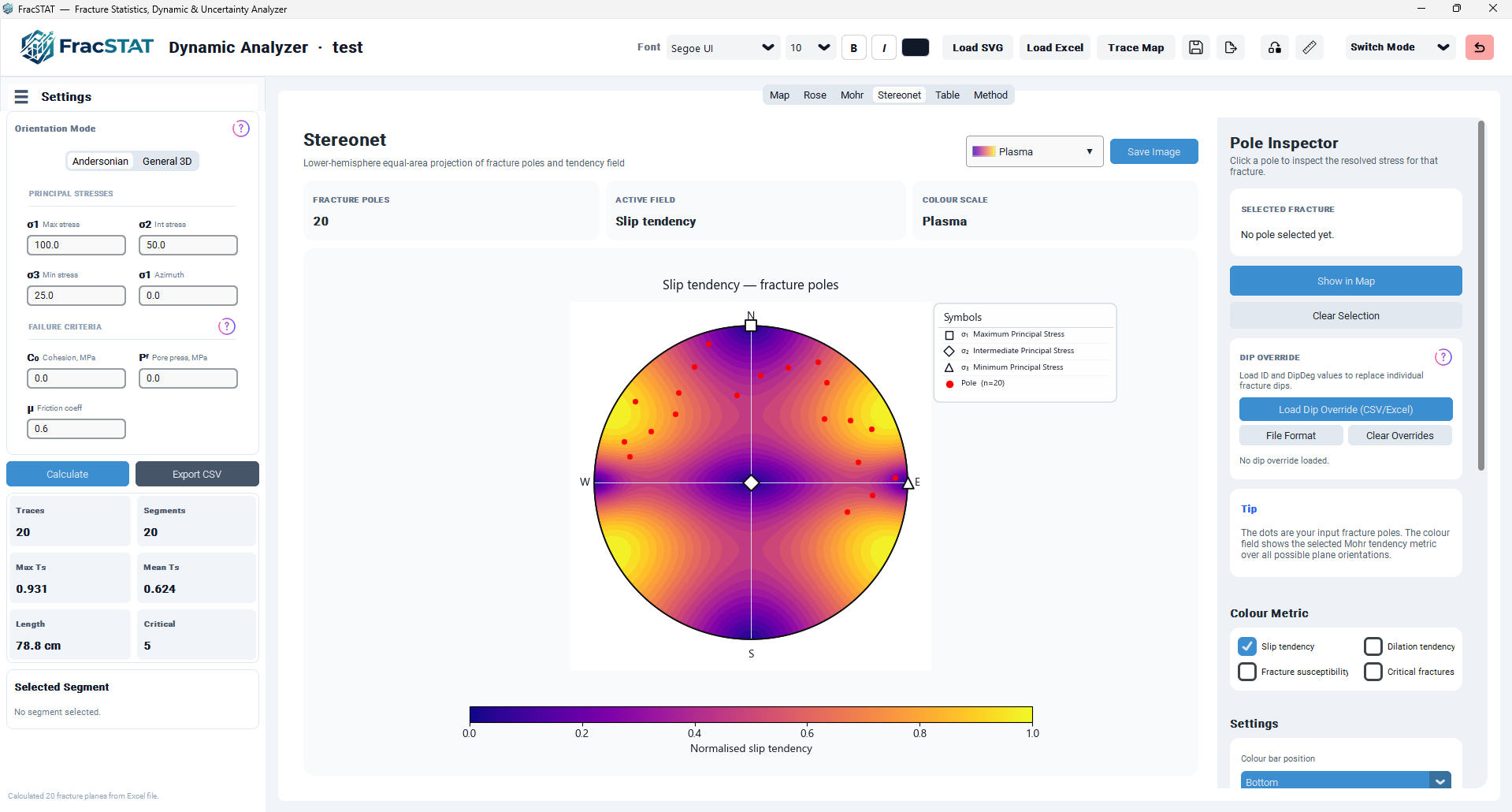
The tab is organised as a two-column layout inside the Dynamic Analyzer's tabbed workspace. The left (main) column is a rounded card containing a header, a row of three summary tiles, and the plotting canvas. The right column is a scrollable panel containing the Pole Inspector, the dip-override loader, a usage tip, the Colour Metric selector, and the full Settings section.
1.1 Header and Summary Tiles
The header carries the title "Stereonet", a one-line description ("Lower-hemisphere equal-area projection of fracture poles and tendency field"), a colour-scale dropdown (shared with the Mohr tab, see Section 5.1), and a Save Image button. Beneath the header, three tiles summarise, at a glance, the current state of the plot:
| Tile | Displayed Value | Update Trigger |
|---|---|---|
| Fracture poles | Count of segments/planes currently plotted (len(self.results)) | Every redraw of the stereonet |
| Active field | Name of the currently selected colour-by attribute (e.g. "Slip tendency") | Whenever the Mohr/Stereonet shared metric checkboxes change |
| Colour scale | Name of the selected Matplotlib colormap (e.g. "Plasma") | Whenever the colormap dropdown changes |
1.2 Main Plot Canvas
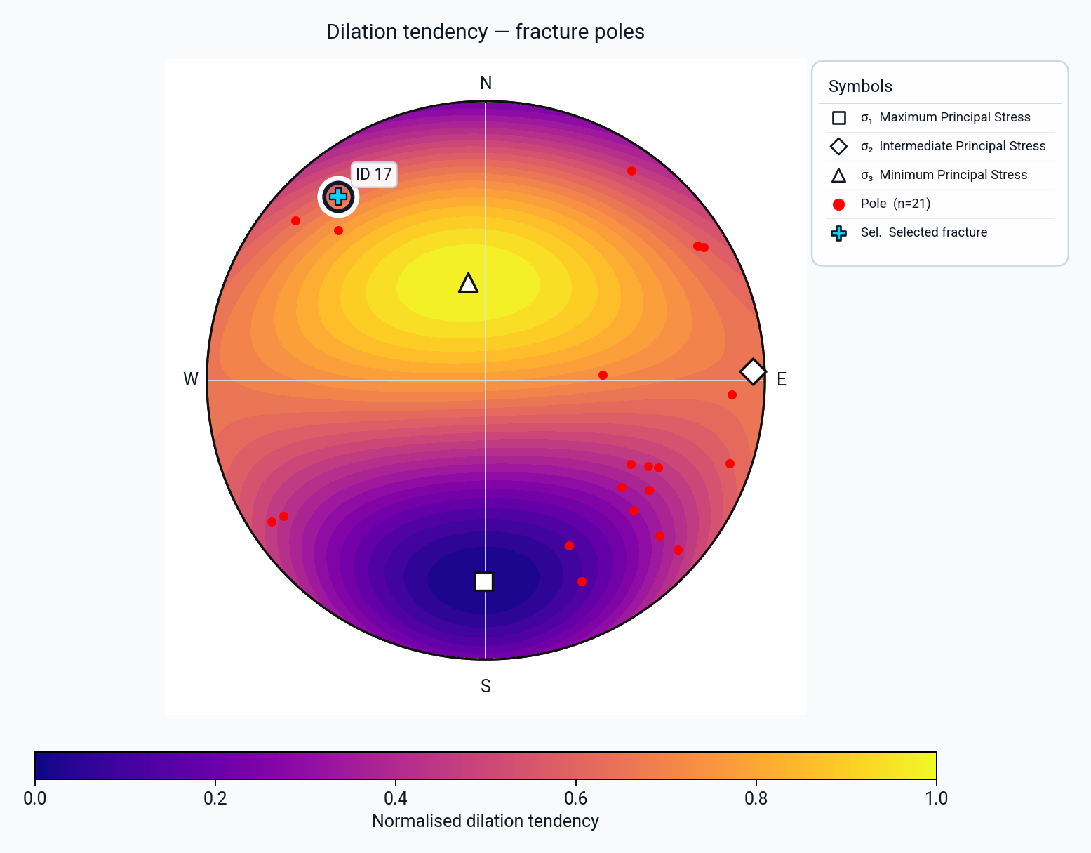
The plot canvas is a single square Matplotlib Axes hosting: the equal-area primitive circle, optional grid rings/degree ticks, the N/E/S/W (or numeric) perimeter labels, the continuous tendency field (a filled Delaunay triangulation), the fracture poles (a scatter collection with picking enabled), optional great-circle planes, the three principal-stress markers, a draggable "Symbols" legend box, and — when a colour metric is active — a colour bar. A dedicated horizontal Axes beneath the main plot hosts the colour bar so that its position and thickness can be adjusted independently of the main circle's aspect ratio.
1.3 Pole Inspector Panel
The right panel opens with a short instructional paragraph ("Click a pole to inspect the
resolved stress for that fracture.") followed by a bordered card labelled SELECTED FRACTURE.
This card is blank ("No pole selected yet.") until the user clicks a pole or a row in the
Table tab; it is populated by update_stereonet_selection_panel(), described in
Section 3.6.
1.4 Navigation and Selection Controls
| Control | Type | Action |
|---|---|---|
| Show in Map | Button | Switches the workspace to the Map tab with the same segment ID highlighted (select_segment(..., switch_to_map=True)). |
| Clear Selection | Button | Deselects the current pole across Map, Mohr, Table, and Stereonet simultaneously (clear_selection()). |
| Dip Override card | Composite widget | Shared control (built by _build_dip_override_card) for loading a CSV/Excel dip-override file; described in Section 5.6. |
2. Data Input and Preprocessing
The Stereonet Tab performs no file I/O of its own. All orientation and stress data arrive
pre-computed in self.results, a pandas DataFrame produced by
calculator.run_calculation() once the user has loaded an SVG trace map or an
Excel/CSV orientation table and pressed Calculate (or edited any stress parameter). The
columns the Stereonet Tab reads are summarised below.
| Column | Source | Role in Stereonet Tab |
|---|---|---|
StrikeDeg | SVG geometry or preset Excel strike | Converted to pole trend (Section 3.2); read modulo 360° to preserve dip direction. |
DipDeg | SVG default dip / Excel preset dip / per-ID override | Converted to pole plunge via the equal-area radius formula (Section 3.1). |
ID | Row index assigned in run_calculation() | Used for pole picking (on_stereonet_pick) and cross-tab selection. |
SlipTendencyNorm | Wallace–Bott resolved shear/normal ratio, normalised by the theoretical maximum | One of four selectable colour-by metrics. |
DilationTendency | (σ1 − σn)/(σ1 − σ3) | One of four selectable colour-by metrics. |
FractureSusceptibility | σn − Pf − (τ − C0)/μ | One of four selectable colour-by metrics. |
CriticalStateValue | Four-tier friction-demand classification (0–3) | One of four selectable colour-by metrics; forces a discrete four-colour scale. |
EffectiveSigmaN, Tau | Resolved normal/shear stress at the current stress tensor | Displayed verbatim in the Pole Inspector card. |
2.1 Dip Override Injection
Before strikes and dips reach the plotting routine, the tab checks self.results
for an ID column and a non-empty static/dynamic dip_overrides mapping (populated
by the shared Load Dip Override control, see Section 5.6). Where an
override exists for a given ID, the DipDeg value is replaced; rows without an
override keep their original dip. Because the dip determines the pole's radial position on
the equal-area net, this override changes where — but not whether — the corresponding pole
is drawn.
2.2 Dip-Direction Correction
Legacy Excel imports and any workflow that supplies a DipDirection column
trigger an additional correction: wherever DipDirection is finite, the strike
used for pole placement is recomputed as (DipDirection − 90°) mod 360°, overriding the raw
StrikeDeg value for that row only. This keeps the stereonet consistent with data
sources that report dip azimuth directly rather than strike.
2.3 Validity Filtering
Rows with non-finite strike or dip (e.g. produced by malformed input rows that survived upstream validation) are excluded from the plotted set via a combined finite-value mask; dip is additionally clipped to the physically valid 0–90° range before any trigonometric evaluation. If the filtered set is empty, the tab falls back to an explanatory empty state (Section 6.4) rather than attempting to draw.
3. Mathematical Background
3.1 Lower-Hemisphere Equal-Area (Schmidt) Projection
Every point plotted on the net — poles, principal-stress axes, and great-circle traces of planes — uses the Lambert equal-area, lower-hemisphere convention standard in structural geology (Ragan, 2009). For a line with trend θ (measured clockwise from north) and plunge δ (measured downward from horizontal), the projected radius r and Cartesian plotting coordinates (x, y) are:
The primitive circle (the outer boundary of the net) corresponds to r = 1, i.e. a horizontal line (δ = 0°); the centre of the net corresponds to a vertical line (δ = 90°). This projection preserves area, which is what permits density-style visual comparison between clusters of poles without the areal distortion of a stereographic (equal-angle) projection (Vollmer, 1995; Cardozo and Allmendinger, 2013).
3.2 Pole Position from Strike and Dip
A fracture plane is fully described by its strike (azimuth of the horizontal line contained in the plane, right-hand-rule convention) and dip (angle below horizontal, measured perpendicular to strike). Its pole is the line perpendicular to the plane, and by the right-hand rule its trend is exactly 90° counter-clockwise from the dip-direction, i.e. (Allmendinger et al., 2012):
Substituting pole_plunge into the equal-area radius formula from Section 3.1 gives the specific expression used throughout the module for the pole radius, r = √2 · sin(dip/2), since 90° − pole_plunge = dip. The module deliberately preserves the fully-directed 0–360° form of strike (rather than folding it into the 0–180° fracture convention used by the Rose tab) precisely because the pole position depends on which side of the strike line the plane dips toward; folding the strike would silently collapse two physically distinct dip directions onto a single hemisphere position.
StrikeDeg happens to already be in. Folding strike to 0–180°
upstream throws away which side the plane dips toward — exactly what would collapse poles
onto a single hemisphere instead of the two clusters a correct stereonet should show for the
same data.
3.3 Great-Circle (Plane) Trace
When the "Show all planes" or "Show selected plane only" toggle is enabled, each plane's full great-circle trace is drawn by sweeping a parameter t from 0 to π across the strike and down-dip unit vectors in an East-North-Up basis:
where strike_vector = (sinψ, cosψ, 0), and down_dip_vector = (sin(ψ+90°)cosδ′, cos(ψ+90°)cosδ′, −sinδ′) for strike azimuth ψ and dip δ′. Each swept vector v(t) = (vE, vN, vU) is converted back to a trend/plunge pair via plunge = asin(−vU) and trend = atan2(vE, vN), then projected with the same equal-area radius formula, producing the smooth curved trace characteristic of a dipping plane on an equal-area net (a vertical plane traces a straight diameter; a shallow plane traces a tight loop near the primitive circle).
3.4 Stress Resolution on the Continuous Orientation Field
The coloured field underlying the poles is not derived from the loaded fracture data at all — it is the theoretical response of the current stress tensor evaluated across a dense, regular grid of colatitude and trend values covering the entire lower hemisphere (64 colatitude steps × 128 trend steps, avoiding the exact pole and equator to prevent singularities). For each grid orientation the unit normal vector components in an East/North/Up basis are:
These are projected onto the three principal-stress axis directions (Section 3.5) to obtain direction cosines c0, c1, c2, from which the resolved normal and shear stress follow the standard Cauchy stress-transformation identities (Jaeger et al., 2007):
From these, the four selectable field values are computed grid-point-by-grid-point exactly as in the Mohr tab:
| Metric | Formula | Normalisation |
|---|---|---|
| Slip tendency (normalised) | Ts = τ / max(σn, 10⁻¹²) | Divided by the closed-form theoretical maximum Ts,max = (σ1 − σ3) / (2·√(σ1·σ3)), not by the largest value on the grid, so the field matches the per-fracture SlipTendencyNorm column exactly (Section 7.1). |
| Dilation tendency | Td = (σ1 − σn) / (σ1 − σ3) | Already dimensionless, 0–1 by construction. |
| Fracture susceptibility | Sf = σn − Pf − (τ − C0)/μ | Raw form displayed in stress units (e.g. MPa). The normalised form is rescaled against the loaded fractures' Sf minimum and maximum and then inverted, 1 − (Sf − min)/(max − min), so the least stable orientations map to 1.0, matching the inversion in calculator.py; the field is set to 0 everywhere if that range collapses below 10⁻¹². |
| Critical fractures | threshold_ratio = [(τ − C₀) / (σn − Pf)] / μ, banded to 0=Stable, 1=Near Critical, 2=Critical, 3=Unstable at the 50%/75%/100% thresholds | Discrete four-colour scale (Stable / Near Critical / Critical / Unstable). |
This same field-evaluation logic is shared with the Mohr tab's own contour computation, ensuring the two diagrams are always mutually consistent for a given stress state — a fracture that appears deep in the "hot" colour region on the stereonet will also plot on or beyond the Coulomb envelope in the Mohr diagram.
3.5 Principal Stress Axis Construction
Two stress-orientation modes are supported, matching the Mohr and Map tabs. In Andersonian mode (Anderson, 1951), σ1 is horizontal along the entered azimuth, σ2 is exactly vertical, and σ3 is horizontal and perpendicular to σ1:
where α is the σ1 azimuth in radians. This is the strike-slip Andersonian regime
(Sv = σ2) — the only one the simplified mode builds, and now named explicitly as the
default vertical_axis="sigma2" of andersonian_principal_axes(), which
also accepts "sigma1" (normal faulting, Sv = σ1) and "sigma3"
(reverse/thrust, Sv = σ3). Note that the Uncertainty Analyzer's default is the
opposite convention, Sv = σ3, so a stereonet built here and a slip-tendency
distribution built there are not directly comparable unless the same regime is chosen in both.
In General 3-D mode, the fully general routine
principal_stress_axes_fracstat(σ1_trend, σ1_plunge, σ3_trend) is used: σ1 is
built directly from its own trend/plunge; σ3's plunge is solved so that σ3 is exactly
orthogonal to σ1 (using the supplied σ3 trend as a starting horizontal direction and
re-normalising); and σ2 is obtained as the cross product σ3 × σ1, ensuring a mutually
orthogonal right-handed frame from only three independent input angles. For plotting
purposes, axis_to_trend_plunge() converts each resulting axis back into a
trend/plunge pair using a downward-pointing-line convention with a tolerance-based sign
correction (±10⁻⁹) that guards against floating-point noise spuriously flipping a
near-horizontal axis by 180°.
3.6 Kinematic (Wallace–Bott) Consistency for Focal Mechanisms
The Wallace–Bott hypothesis holds that slip on a pre-existing plane occurs parallel to the resolved shear traction on that plane (Wallace, 1951; Bott, 1959), so the angular difference between the observed and predicted slip directions is a direct test of whether an observed slip event is compatible with the assumed stress tensor. When a loaded dataset is a focal-mechanism (earthquake) file supplying a rake/slip value, the Stereonet Tab shares the same slip-tendency, dilation-tendency, and fracture-susceptibility metrics computed for the nodal plane; the underlying calculator additionally resolves the shear traction along the observed slip vector and reports a Rake Misfit, but this Wallace–Bott diagnostic is displayed in the Pole Inspector text panel (shared with the Map and Mohr tabs) rather than as a stereonet colour metric or a Table-tab column: the inspector prints the signed resolved shear along the slip vector, the predicted rake, and the misfit, labelling the latter "consistent" at ≤ 30° and "inconsistent" above it.
fault_basis_vectors(strike, dip) in an
(East, North, Up) frame: the unit strike vector ŝ = (sin strike, cos strike, 0), the
down-dip vector d̂ = (sin·cos, cos·cos, −sin) taken along the dip direction
strike + 90°, and the upward pole n. Because the traction is assembled from
compression-positive stress magnitudes, the physical (tension-positive) shear traction acting on
the hanging wall is the negative of the in-plane traction component,
and the observed slip direction follows the
Aki and Richards (1980, §4.2) rake convention
(0° left-lateral, +90° reverse/up-dip, 180° right-lateral, −90° normal/down-dip):
predicted_rake converts a down-dip component into
the up-dip-positive Aki and Richards (1980) sense, so that
observed and predicted rakes are compared in
the same convention; and the modulo-360 wrap folds the difference into 0–180°, so a misfit is
never reported as, say, 350° when the true angular separation is 10°.
colatitude = np.linspace(.01, np.pi / 2 - .01, 64)
trend = np.linspace(0, 2 * np.pi, 128, endpoint=False)
colatitude, trend = np.meshgrid(colatitude, trend)

normal_east  = np.sin(colatitude) * np.sin(trend)
normal_north = np.sin(colatitude) * np.cos(trend)
normal_up    = -np.cos(colatitude)
s1, s2, s3 = stress["sigma1"], stress["sigma2"], stress.get("sigma3", stress["sigma2"])

sigma_n = s1*c0**2 + s2*c1**2 + s3*c2**2
traction_sq = s1**2*c0**2 + s2**2*c1**2 + s3**2*c2**2
tau = np.sqrt(np.maximum(traction_sq - sigma_n**2, 0.0))

if column.startswith("SlipTendency"):
    raw = tau / np.maximum(sigma_n, 1e-12)
    if column == "SlipTendencyNorm":
        # Closed-form theoretical maximum, NOT raw.max() over the grid.
        denom = 2.0 * np.sqrt(max(s1 * s3, 1e-12))
        tsmax = max((s1 - s3) / denom, 1e-12)
        field_values = raw / tsmax
    else:
        field_values = raw
elif column == "DilationTendency":
    field_values = (s1 - sigma_n) / max(s1 - s3, 1e-12)
elif column.startswith("FractureSusceptibility"):
    raw_values = sigma_n - stress["pore_pressure"] - (tau - stress["cohesion"]) / max(stress["friction"], 1e-12)
    if column == "FractureSusceptibilityNorm" and not self.results.empty:
        sf_min = float(self.results["FractureSusceptibility"].min())
        sf_max = float(self.results["FractureSusceptibility"].max())
        sf_range = sf_max - sf_min
        # Inverted: a SMALLER Sf is MORE susceptible, so it maps to 1.0.
        field_values = (np.zeros_like(raw_values) if abs(sf_range) < 1e-12
                        else 1.0 - (raw_values - sf_min) / sf_range)
    else:
        field_values = raw_values
else:
    field_values = (tau >= stress["cohesion"] + stress["friction"]*(sigma_n - stress["pore_pressure"])).astype(float)

radius = np.sqrt(2) * np.sin(colatitude / 2)
field_x, field_y = (radius*np.sin(trend)).ravel(), (radius*np.cos(trend)).ravel()
Simplified excerpt of _draw_stereonet(), showing the analytic 64×128 grid construction and the four selectable field-value formulas.
4. Algorithms
4.1 Field-Contouring Algorithm
- Build a meshgrid of 64 colatitude values (0.01 to π/2 − 0.01) by 128 trend values (0 to 2π, endpoint excluded).
- Compute the unit normal-vector components at every grid node (Section 3.4).
- Project each normal onto the active principal-stress frame to obtain direction cosines.
- Evaluate σn and τ, then the selected scalar field value (Ts, Td, Sf, or the four-tier critical-fracture-state classification).
- Convert every grid node's (colatitude, trend) into equal-area (x, y) plotting coordinates using the same radius formula as the poles.
- Triangulate the resulting scattered point cloud with
matplotlib.tri.Triangulationand render it withax.tricontourfat 24 discrete colour levels (or, for the Critical fractures metric, at the fixed boundary levels [-0.5, 0.5, 1.5, 2.5, 3.5] so the four states render as crisp bands rather than a smoothed gradient).
Because the triangulation is built once per redraw directly from the analytic grid (not from the sparse, irregularly spaced fracture poles), the field is smooth and continuous regardless of how many or how few fractures are actually loaded — it represents the theoretical stress response, not an interpolation of the data.
4.2 Pole Placement and Picking
Poles are computed vectorised across the entire filtered DataFrame using NumPy: pole_trend =
(strike − 90°) mod 360° and pole_radius = √2·sin(dip_rad/2), then x = radius·sin(trend_rad), y
= radius·cos(trend_rad). The resulting scatter artist is registered as a matplotlib "pickable"
object with a pick radius of 6 points; a click within that radius fires
on_stereonet_pick, which maps the picked index back to a row of
self.results and calls the shared select_segment() method — the
same selection entry point used by the Map, Mohr, and Table tabs, guaranteeing the four views
never fall out of sync.
4.3 Draggable Symbol Index
The legend ("Symbols") box in the lower-right corner of the plot is not a native Matplotlib
Legend but a hand-built composite of a FancyBboxPatch, text labels, and scatter
markers, all scaled by the current global font size relative to a 10-pt baseline. This custom
construction allows the box to be interactively repositioned when "Move Elements" mode is
active in the workspace header: on_stereo_press hit-tests the box's stored (x0,
y_top, width, height) footprint in axes-fraction coordinates; on_stereo_motion
translates the anchor by the mouse displacement (expressed as a fraction of the axes' pixel
bounding box) and calls a cheap redraw routine (_redraw_stereo_symbol_index) that
repositions only the index artists rather than re-running the full stereonet draw, which
would be considerably more expensive because it would re-evaluate the entire
field-contouring grid. The anchor position persists across redraws in
self._stereo_symbol_index_pos, and defaults to just outside the plot's own axes
bounding box (x0 = 1.02) so it never overlaps the stereonet circle regardless of how large
the font grows.
4.4 Colour-Bar Layout Algorithm
Depending on the selected Colour bar position (Bottom/Top/Left/Right/None), the routine computes a rectangle for the dedicated colour-bar Axes (in figure-fraction coordinates) sized by the user-configured thickness and length fractions, and simultaneously repositions the main stereonet Axes so the circle stays centred and undistorted next to the bar. The Diagram Scale slider (Section 5.3) is applied multiplicatively to both width and height of the main Axes about the same centre point used for the colour-bar layout, so enlarging or shrinking the diagram never displaces its centre.
4.5 Selected-Pole Highlight and Selected-Plane Trace
When self.selected_segment_id is not None, a three-layer halo
(white ring, dark ring, coloured "P" plus-marker) is drawn over the corresponding pole and
annotated with its ID. If "Show Selected Plane" is enabled, the great-circle trace of that
one plane (Section 3.3) is additionally drawn in the user-selected highlight colour, letting
the analyst see the full orientation of a single fracture of interest without cluttering the
net with every plane in the dataset.
5. Settings and Controls
All settings are held in dedicated CTk variables, lazily initialised the first time the tab
is built (_stereo_init_vars) so that re-opening the tab, switching projects, or
restoring a saved session never silently resets a control the user had already configured.
Every control below triggers _draw_stereonet() on change unless noted otherwise.
5.1 Colour Metric (shared with the Mohr Tab)
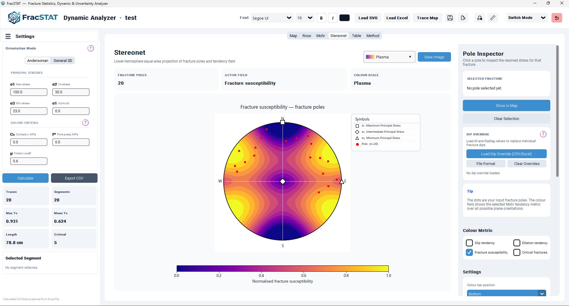
Four checkboxes — Slip tendency, Dilation tendency, Fracture susceptibility, Critical fractures —
are mutually exclusive (selecting one automatically clears the others) and are bound to the
same mohr_slip_var / mohr_dilation_var / mohr_fracture_var
/ mohr_critical_var variables used by the Mohr tab, via the shared
change_mohr_metric() callback. This deliberate sharing means changing the active
metric on either tab updates both simultaneously; the Stereonet Tab does not maintain its own
independent copy of the "Critical fractures" state, so the four-tier classification and its
thresholds are always identical between the two tabs for a given stress state.
5.2 Settings Card — General Appearance
| Control | Widget | Default | Effect |
|---|---|---|---|
| Colour bar position | Dropdown | Bottom | Bottom / Top / Left / Right / None; repositions colour bar and rescales the main diagram (Section 4.4). |
| Outer BG | Colour swatch | #F8FAFC | Figure (outer canvas) background colour. |
| Inner BG | Colour swatch | #FFFFFF | Stereonet Axes background colour. |
| CBar Width | Numeric entry | 0.03 | Colour-bar thickness as a fraction of the figure. |
| CBar Length | Numeric entry | 0.64 | Colour-bar length as a fraction of the figure. |
5.3 Settings Card — Pole and Border Styling
| Control | Widget | Default | Effect |
|---|---|---|---|
| Pole Color | Colour swatch | #FF0000 | Fill colour of pole markers when solid-colour mode effectively applies (no metric selected uses this colour for the index; poles themselves are always coloured by the active field when a metric is chosen). |
| Pole Border | Colour swatch | #FF0000 | Marker edge colour. |
| Border Width | Numeric entry | 0.3 | Marker edge line width, points. |
| Selected Pole | Colour swatch | #00D4FF | Highlight colour used for the selected pole's plus-marker and, if enabled, the selected plane's great-circle trace. |
| Boundary Color | Colour swatch | #111111 | Colour of the primitive circle and (if enabled) the 30° tick marks. |
| Boundary Width | Numeric entry | 1.2 | Line width of the primitive circle. |
| Pole Shape | Dropdown | Circle | Circle / Diamond / Square / Triangle Up / Star / Cross — maps to Matplotlib marker codes o / D / s / ^ / * / X. |
| Pole Size | Numeric entry | 24 | Marker area in points² (matplotlib scatter s parameter). |
| Diagram Scale | Numeric entry | 1.0 | Multiplicative scale factor applied to both width and height of the main Axes about its current centre (Section 4.4). |
| Custom Title | Text entry | (blank) | Overrides the auto-generated title "<metric> — fracture poles". |
5.4 Settings Card — Toggles
| Toggle | Default | Effect |
|---|---|---|
| Show N-S / E-W Lines | On | Draws the two crosshair diameters through the net centre. |
| Show Selected Plane | Off | Draws the great-circle trace of only the currently selected fracture, in the Selected Pole colour. |
| Show All Poles | On | Toggles visibility (and pickability) of the entire pole scatter collection; turning it off disables clicking to select a fracture from the stereonet. |
| Show All Planes | Off | Draws every loaded fracture's great-circle trace at low opacity (alpha = 0.25), useful for visualising the overall fabric of dipping surfaces rather than just their poles. |
5.5 Reset Defaults
The Reset Defaults button (_stereo_reset_defaults) restores every one of the
settings above to its factory value in a single action and immediately redraws — useful
after exploratory styling changes before generating a publication figure.
5.6 Dip Override Card
Shared with every other Dynamic Analyzer tab that displays per-segment dip (Mohr, Map, Stereonet), this card provides: a "Load Dip Override (CSV/Excel)" button that opens a file dialog and parses an ID/DipDeg table (column names are matched case-insensitively after stripping non-alphanumeric characters, so "Dip Deg", "dip_deg", and "DipDeg" are all accepted); a "File Format" button that opens a hover preview showing the exact two-column layout expected; and a "Clear Overrides" button. Overrides are validated to lie within 0–90° before being accepted, and are keyed by the same one-based ID used in the Table tab, so an override file exported from one project session can be reused directly against another session with an identical segment count and ordering.
6. Internal Workflow
6.1 Build Sequence (_build_stereonet_tab)
- Initialise all settings variables (Section 5) and the draggable symbol-index state (position, drag flag, artist list).
- Construct the outer rounded card, header row (title, subtitle, colour-scale dropdown, Save Image button), and the three summary tiles.
- Construct the plot card containing the Matplotlib Figure/Axes pair and its dedicated colour-bar Axes, then wrap it in a
FigureCanvasTkAggand bindpick_event,button_press_event,motion_notify_event, andbutton_release_eventhandlers. - Construct the right-hand scrollable panel: Pole Inspector heading and instructions, the Selected Fracture card, Show in Map / Clear Selection buttons, the Dip Override card, a Tip card, the Colour Metric checkboxes, and the full Settings card tree.
- Call
_draw_stereonet()once to render the initial (likely empty) state.
6.2 Draw Sequence (_draw_stereonet)
- Read and validate every styling variable (colours, widths, sizes), falling back to a safe default on any parse failure so a malformed numeric entry never crashes the redraw.
- Clear the Axes and colour-bar Axes; reset the fixed aspect-1 limits (−1.15 to 1.15 in both axes) and hide the default tick marks.
- Draw the primitive circle, optional crosshairs, and either the 30° perimeter tick/degree-label ring (when "Show Selected Plane" is on) or the plain N/E/S/W labels.
- If
self.resultsis empty or no stress has been calculated, populate the summary tiles with placeholder text, render the title "Stereonet", and return early (Section 6.4). - Resolve the active colour metric (falling back to Slip tendency if none is checked), update the three summary tiles, and build the principal-stress axis frame (Section 3.5).
- Evaluate the continuous tendency field over the analytic grid (Sections 3.4/4.1) and render it with
tricontourf; redraw the primitive circle on top so the field never bleeds past the net's boundary. - Compute pole_trend/pole_radius for every valid row (Section 4.2); optionally draw every plane's great circle first (so poles render on top), then draw the pole scatter (respecting "Show All Poles").
- If a segment is selected, draw its highlight halo, ID annotation, and (optionally) its individual great-circle trace.
- Attach the ScalarMappable-driven colour bar per the chosen position (Section 4.4), draw the three principal-stress axis symbols, and render the draggable Symbols index (Section 4.3).
- Apply the custom or auto-generated title and request an idle redraw of the canvas (
draw_idle).
6.3 Selection Synchronisation
select_segment() (defined at the SlipTendencyApp level, not within
this mixin) is the single choke point through which a pole click, a Table row click, or a
Mohr-diagram click all flow. It updates self.selected_segment_id, calls
update_stereonet_selection_panel() to refresh the Pole Inspector card, and then
calls _draw_stereonet() (among the other tabs' own redraw methods) so the newly
selected pole's halo appears immediately, without the user needing to manually refresh.
6.4 Empty and Degenerate States
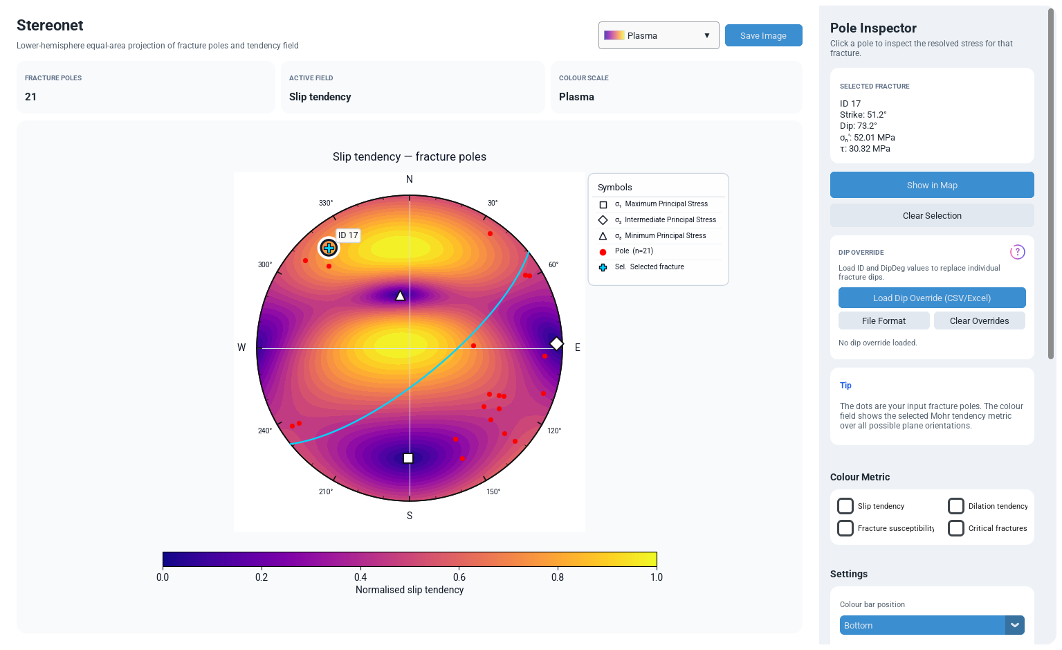
Two distinct "nothing to show" conditions are handled: (a) no data loaded at all, or no stress tensor yet calculated — the tiles reset to "0" / "Slip tendency" / the current colour-scale name, and the title reads simply "Stereonet"; and (b) data loaded but every row fails strike/dip validity filtering (Section 2.3) — handled by the same early-return path since the filtered array would again be empty. In both cases the primitive circle, crosshairs, and cardinal labels are still drawn, so the net's geometry frame of reference is always visible even with no data.
7. Statistical Methods
The Stereonet Tab itself performs no descriptive statistics beyond a simple count (the "Fracture poles" tile). All quantitative summary statistics for the loaded fracture population (mean strike, dominant azimuth bin, dispersion, etc.) belong to the Rose tab; the Stereonet Tab is instead the qualitative / visual complement, letting the analyst judge cluster tightness, bimodality, or great-circle girdle patterns by eye against the coloured stress field. Where quantitative rigor is required — e.g. testing whether a pole cluster is statistically consistent with the maximum-Ts orientation predicted by the stress tensor, which calls for the eigenvalue and confidence-cone machinery of spherical statistics (Fisher et al., 1987) — the underlying field values (Ts, Td, Sf) available per-fracture in the Table tab and per-orientation on the continuous grid used here can be exported and analysed externally (Section 9.3).
7.1 Theoretical Maximum Normalisation
The normalised slip-tendency field divides every grid value of τ/σn by a closed-form constant rather than by the largest value that happens to appear on the 64×128 grid:
This is the exact theoretical maximum of τ/σn over every possible plane orientation for a
diagonal principal-stress tensor, and it depends on σ1 and σ3 alone — not on σ2, not on the
principal-axis orientation, and not on the discretisation of the grid. It is the same constant the
calculator module's _theoretical_max_slip_tendency() uses for the per-fracture
SlipTendencyNorm column, so the stereonet field and the Table/Map/Mohr colouring are
numerically consistent by construction rather than only approximately. Taking the grid maximum
instead would make the normalisation depend on the mesh: the grid stops short of the poles
(colatitude runs 0.01 to π/2 − 0.01 rad) and samples azimuth in 128 steps, so it need not contain
the optimally oriented plane.
_theoretical_max_slip_tendency() clamps it proportionately to the stress
magnitude, at 10⁻⁶·max(σ1², 1). For ordinary compressive states with σ3 > 0 the two agree
exactly; only in the degenerate σ3 ≤ 0 case can the field and the per-fracture column be scaled
differently, and in that regime neither normalised value should be read quantitatively.
8. Visualization Components
| Component | Matplotlib Primitive | Purpose |
|---|---|---|
| Primitive circle | ax.plot on a 361-point unit circle | Defines the projection boundary (equator of the lower hemisphere). |
| Grid rings / degree ticks | ax.plot radial tick segments + ax.text | Optional 30° azimuth reference marks around the perimeter, shown only when "Show Selected Plane" is enabled. |
| N-S / E-W crosshair | ax.plot two diameters | Quick visual reference for cardinal directions. |
| Tendency field | ax.tricontourf over a Delaunay triangulation | Continuous colour-coded stress-response surface across the whole hemisphere. |
| Fracture poles | ax.scatter (pickable) | Discrete data points; colour and/or shape configurable. |
| Great-circle plane traces | ax.plot (per-plane parametric sweep) | Optional visualisation of full plane orientation, not just its pole. |
| Principal-stress markers | ax.scatter with square/diamond/triangle markers | σ1 (square), σ2 (diamond), σ3 (triangle) axis positions. |
| Selected-pole halo | Two concentric ax.scatter rings + plus-marker | Draws attention to the currently selected fracture. |
| Symbols index | Custom FancyBboxPatch + text/markers | Draggable legend explaining every marker on the plot (Section 4.3). |
| Colour bar | fig.colorbar bound to a ScalarMappable | Quantitative scale for the active tendency metric. |
9. Advanced Features
9.1 General 3-D Stress Orientation Mode
When the sidebar's Orientation Mode tab is set to General 3D, the Stereonet Tab automatically
re-derives the principal-stress axis positions using
principal_stress_axes_fracstat() rather than the simplified Andersonian
formulas, so the three principal-stress markers correctly reflect fully general
(non-Andersonian) stress-field orientations such as oblique-slip regimes.
9.2 Draggable Symbols Index
Described in Section 4.3. This is a workspace-wide "Move Elements" feature: when enabled from the header, every draggable overlay across all Dynamic Analyzer tabs (Mohr's Symbols index, the Rose tab's legend, and this Stereonet index) becomes repositionable by click-and-drag, letting the analyst tailor figure layout before exporting an image for a report.
9.3 Cross-Tab Data Sharing and Export
Because the Stereonet Tab reads directly from self.results, any change made
elsewhere in the workspace — loading a different data source, editing the stress tensor,
applying a dip override, or switching units — is reflected here on the very next redraw with
no separate synchronisation step. The Save Image toolbar button exports the current
stereonet figure (including whatever position the Symbols index has been dragged to) as a
high-resolution PNG through the shared save_plot_image() routine, using the
export DPI configured in Settings and a filename that encodes the project name, plot name,
active metric, and a timestamp.
9.4 Focal-Mechanism Aware Pole Placement
For Excel/CSV files following the Global CMT-style focal-mechanism format (Lat, Lon, FP1/FP2
Strike/Dip, optional Slip/Rake), each nodal plane becomes its own row in
self.results and is plotted here exactly like any other fracture plane, letting
seismological nodal-plane populations be compared on the same equal-area net and against the
same resolved-stress colour field as outcrop- or map-derived fracture data.
10. Performance Optimization
10.1 Analytic Grid Sizing
The continuous tendency field is evaluated on a fixed 64×128 grid (8,192 nodes) rather than scaling with the number of loaded fractures. This keeps the triangulation and contour-fill cost constant and fast even for datasets containing many thousands of segments, since the expensive part of the redraw is the field, not the (fully vectorised) pole scatter.
10.2 Vectorised Pole Computation
Strike, dip, pole trend, and pole radius are all computed with NumPy array operations across the entire filtered DataFrame in a single pass rather than a per-row Python loop, so plotting thousands of poles remains a near-constant-time operation relative to redrawing the field.
10.3 Cheap Redraw Path for Dragging
As noted in Section 4.3, dragging the Symbols index calls
_redraw_stereo_symbol_index(), which removes and rebuilds only the index's own
artists (cached from the most recent full draw's arguments in
self._stereo_index_last_args) rather than invoking the full
_draw_stereonet() pipeline. This avoids recomputing the 8,192-node field and
re-triangulating on every mouse-move event during a drag, which would otherwise make the
interaction feel sluggish.
10.4 Idle-Draw Scheduling
All redraws finish with self.stereo_canvas.draw_idle() rather than a blocking
draw(), deferring the actual GPU/CPU rendering work to the next idle slot in
Qt's event loop so rapid successive setting changes (e.g. typing in a numeric field) do
not each force an immediate, separate render pass.
11. Practical Examples
11.1 Example — Checking Orientation-Stress Compatibility
- Load an SVG trace map or Excel orientation table, then enter or confirm the principal stress magnitudes and orientation on the sidebar.
- Open the Stereonet Tab and leave Slip tendency selected as the colour metric.
- Observe whether the plotted poles cluster inside the "hot" (high-Ts) region of the field, near the perimeter close to the σ1 marker's perpendicular great circle, or in the "cool" low-Ts region near σ3.
- If most poles fall in a cool region, the current stress field is unlikely to be reactivating that fracture set, prompting a re-examination of either the assumed stress orientation or the possibility that the fractures are inherited from an earlier tectonic event.
11.2 Example — Verifying a Dip Override
- Load a dip-override CSV containing ID and DipDeg columns for a subset of segments.
- Compare the Stereonet Tab before and after loading: overridden poles will move radially (their trend is unchanged; only their distance from the centre, governed by dip, changes).
- Use the Show in Map button after selecting an overridden pole to confirm the correct segment was affected.
11.3 Example — Comparing Fracture Sets Against a Focal Mechanism Catalogue
- Load a Global CMT-style focal-mechanism Excel/CSV file alongside (in a separate session) or instead of an outcrop dataset.
- Enable "Show All Planes" to visualise the family of nodal-plane great circles, then toggle Critical fractures as the colour metric to see which nodal planes fall into the Critical or Unstable bands under the entered regional stress tensor.
12. Geological Interpretation
The equal-area stereonet is one of the most information-dense diagrams available to a structural geologist because it simultaneously encodes plane orientation (via pole position) and, in this module's stress-aware variant, the mechanical favourability of every conceivable orientation (via the continuous colour field). Several interpretive principles follow directly from the plotted geometry:
- Poles near the primitive circle correspond to steeply dipping planes; poles near the centre correspond to shallow, near-horizontal planes.
- A tight cluster of poles indicates a single, well-defined fracture set (consistent formation mechanism and stress history); a girdle (poles distributed along a great circle) suggests folding or a rotational deformation history superimposed on an originally more uniform set.
- Poles coinciding with the high-Ts (hot) region of the field, typically forming two conjugate bands roughly 20–30° from the σ1 direction depending on the friction coefficient μ, are the orientations most favourable for shear reactivation under the current stress state — classic Andersonian conjugate shear-fracture geometry (Anderson, 1951; Morris et al., 1996).
- Poles coinciding with high dilation tendency (near σ3) are those most favourable for tensile opening or hydraulic-fracture propagation, relevant for fluid-flow and permeability assessment.
- A Critical fractures colouring that shows most poles in the "Stable" band, despite reasonable stress magnitudes, may indicate either a genuinely low-permeability, mechanically stable fracture network, or that the assumed pore pressure Pf or friction coefficient μ is too conservative for the field setting; poles falling in the "Near Critical" band are worth particular attention, since a modest change in either parameter could shift them into "Critical" or "Unstable" (Sibson, 1985).
- Where the loaded data carry rake information, poles whose Wallace–Bott rake misfit is small are kinematically compatible with the assumed tensor, and a population of consistently small misfits is evidence that the tensor itself is well chosen (Wallace, 1951; Bott, 1959).
Because the field is recomputed live from the sidebar stress tensor, the Stereonet Tab also functions as an exploratory sensitivity tool: adjusting σ1/σ2/σ3 magnitudes, azimuth, pore pressure, or friction and watching how the hot/cool regions shift relative to the fixed pole population is a fast, visual way to bound plausible in-situ stress states consistent with an observed fracture set — a technique closely related to the stress-inversion methods used in borehole image-log interpretation (Barton et al., 1995; Zoback, 2007).
13. Implementation Notes
13.1 Class Structure
StereonetTab is implemented as a Python mixin class, combined with
MapTab, RoseTab, MohrTab, TableTab, and
MethodTab via multiple inheritance into the top-level SlipTendencyApp
class (see dynamic_app.py). This means every method described in this document
(e.g. _draw_stereonet, on_stereo_press) executes with
self bound to the full application instance, giving it direct access to
self.results, self.current_stress,
self.selected_segment_id, and every other tab's shared state without any explicit
message-passing layer.
13.2 Variable Naming and Persistence
All CTk variables use the stereo_ prefix (e.g. stereo_pole_color_var)
to avoid collisions with the identically-purposed variables in the Mohr and Map tabs.
_stereo_init_vars() uses a hasattr guard on every variable so it can
be called safely multiple times (e.g. on every rebuild after a Reset Defaults) without
clobbering a value the user has since changed through some other code path.
13.3 Colour-Scale Sharing
The colormap dropdown at the top of the tab is bound to the same
mohr_colormap_var used by the Mohr tab (via
change_mohr_colour_scale()), and the available colour-scale catalogue (Turbo,
Viridis, Plasma, a custom Parula approximation, etc.) is defined once in the top-level
SlipTendencyApp (_colour_scale_definitions()) and reused across
every tab that offers a colour-scale choice.
13.4 Marker Shape Mapping
The Pole Shape dropdown's human-readable labels are translated to Matplotlib marker codes through a fixed lookup: Circle→o, Diamond→D, Square→s, Triangle Up→^, Star→*, Cross→X. Note this Cross mapping ('X', a filled X) differs slightly from the Mohr tab's own pole-shape dictionary, which maps Cross to 'P' (a plus/filled-cross marker) — a cosmetic difference between the two tabs' otherwise parallel styling systems.
14. Limitations
| Limitation | Description |
|---|---|
| Spatially uniform stress assumption | The continuous tendency field assumes the stress tensor is spatially uniform; it does not account for local stress perturbations near existing fractures, free surfaces, or heterogeneous lithology. |
| Visual clutter for dense datasets | Great-circle plane traces ("Show All Planes") can become visually cluttered for datasets with many hundreds of fractures; the fixed low alpha (0.25) mitigates but does not eliminate this. |
| Non-linear angular compression | The equal-area projection, while area-preserving, still compresses angular relationships non-linearly toward the primitive circle; visual judgements of "cluster tightness" should be corroborated with the quantitative statistics available on the Rose tab. |
| Dip clamping | Dip values are clipped to 0–90°; any input data implying an overturned or otherwise out-of-range dip will be silently clamped rather than rejected. |
| No rake-misfit colour metric | Kinematic (Wallace–Bott) rake-misfit diagnostics for focal-mechanism data appear only in the pole-inspector text panel (τ along slip, predicted rake, misfit); they are not exposed as a Stereonet colour-by metric, and the Table tab's 16 columns do not include them either. |
| No contoured pole density | Poles are plotted as discrete symbols only. No Kamb or Schmidt density contouring of the pole population is available (Vollmer, 1995), so judgements of cluster strength rest on visual inspection of symbol overlap. |
| No orientation statistics or confidence regions | Eigenvalue fabric parameters, mean-vector estimates, and confidence cones about a cluster mean are not computed (Fisher et al., 1987); the tab reports only a pole count (Section 7). |
| No Terzaghi sampling correction | Poles are plotted one per digitised fracture, with no weighting for the orientation bias inherent in sampling planes from a line or a single outcrop face, so an apparent cluster may partly reflect the sampling geometry. |
| Andersonian mode covers one regime | The simplified mode builds only the strike-slip Andersonian configuration (Sv = σ2) by default (Anderson, 1951); normal and thrust regimes require passing a different vertical axis, and the Uncertainty Analyzer defaults to the opposite convention (Section 3.5). |
| Stress tensor is assumed, not inverted | The field is computed from a user-entered tensor. The tab performs no formal stress inversion from the fracture or focal-mechanism population and reports no misfit statistic over the whole data set, so exploring stress states remains a manual, visual exercise (Zoback, 2007). |
15. References
Sources are listed alphabetically within each group. In-text citations throughout this page link to the corresponding entry below.
15.1 Projection and Orientation Analysis
- Allmendinger, R. W., Cardozo, N., & Fisher, D. M. (2012). Structural Geology Algorithms: Vectors and Tensors. Cambridge University Press. https://doi.org/10.1017/CBO9780511920202
- Cardozo, N., & Allmendinger, R. W. (2013). Spherical projections with OSXStereonet. Computers & Geosciences, 51, 193–205. https://doi.org/10.1016/j.cageo.2012.07.021
- Fisher, N. I., Lewis, T., & Embleton, B. J. J. (1987). Statistical Analysis of Spherical Data. Cambridge University Press. https://doi.org/10.1017/CBO9780511623059
- Ragan, D. M. (2009). Structural Geology: An Introduction to Geometrical Techniques (4th ed.). Cambridge University Press. https://doi.org/10.1017/CBO9780511816109
- Vollmer, F. W. (1995). C program for automatic contouring of spherical orientation data using a modified Kamb method. Computers & Geosciences, 21(1), 31–49. https://doi.org/10.1016/0098-3004(94)00058-3
15.2 Stress, Faulting and Reactivation
- Anderson, E. M. (1951). The Dynamics of Faulting and Dyke Formation with Applications to Britain (2nd ed.). Oliver and Boyd, Edinburgh.
- Barton, C. A., Zoback, M. D., & Moos, D. (1995). Fluid flow along potentially active faults in crystalline rock. Geology, 23(8), 683–686. https://doi.org/10.1130/0091-7613(1995)023<0683:FFAPAF>2.3.CO;2
- Jaeger, J. C., Cook, N. G. W., & Zimmerman, R. W. (2007). Fundamentals of Rock Mechanics (4th ed.). Blackwell Publishing, Oxford. ISBN 978-0-632-05759-7.
- Morris, A., Ferrill, D. A., & Henderson, D. B. (1996). Slip-tendency analysis and fault reactivation. Geology, 24(3), 275–278. https://doi.org/10.1130/0091-7613(1996)024<0275:STAAFR>2.3.CO;2
- Sibson, R. H. (1985). A note on fault reactivation. Journal of Structural Geology, 7(6), 751–754. https://doi.org/10.1016/0191-8141(85)90150-6
- Zoback, M. D. (2007). Reservoir Geomechanics. Cambridge University Press. https://doi.org/10.1017/CBO9780511586477
15.3 Fault Kinematics and Focal Mechanisms
- Aki, K., & Richards, P. G. (1980). Quantitative Seismology: Theory and Methods (Vol. 1), §4.2. W. H. Freeman, San Francisco.
- Bott, M. H. P. (1959). The mechanics of oblique slip faulting. Geological Magazine, 96(2), 109–117. https://doi.org/10.1017/S0016756800059987
- Wallace, R. E. (1951). Geometry of shearing stress and relation to faulting. The Journal of Geology, 59(2), 118–130. https://doi.org/10.1086/625831
15.4 Software
- Harris, C. R., Millman, K. J., van der Walt, S. J., Gommers, R., Virtanen, P., Cournapeau, D., … Oliphant, T. E. (2020). Array programming with NumPy. Nature, 585(7825), 357–362. https://doi.org/10.1038/s41586-020-2649-2
- Hunter, J. D. (2007). Matplotlib: A 2D graphics environment. Computing in Science & Engineering, 9(3), 90–95. https://doi.org/10.1109/MCSE.2007.55
Methods statement for the Stereonet Tab. If a figure produced by this tab appears in a publication, the details below are what a reader needs in order to reproduce it, and are what the citations above assume:
Lower-hemisphere equal-area (Schmidt) stereonet of fracture poles, r = √2·sin(dip/2) (Ragan, 2009), for n planes, overlain on a continuous field of the selected stress-tendency metric evaluated on a 64×128 colatitude–trend mesh for σ₁/σ₂/σ₃ = … MPa, P_f = … MPa, C₀ = … MPa and μ = … (Jaeger et al., 2007). Slip tendency normalised by the closed-form theoretical maximum (Morris et al., 1996); principal axes built in Andersonian or general 3-D mode as stated (Anderson, 1951); rake misfits, where reported, follow the Wallace–Bott criterion (Wallace, 1951; Bott, 1959) in the Aki and Richards (1980) rake convention. Implemented in NumPy (Harris et al., 2020) and rendered with Matplotlib (Hunter, 2007). Report the full stress tensor, the orientation mode, the colour metric, and n; note that no pole-density contouring or orientation statistics are computed here (Section 14).