Static CDF Tab
Located at static_analyzer/tabs/static_cdf_tab.py, the CDF Analyzer
tab (implemented as the class StaticCDFTab) is the platform's dedicated module for
quantitative fracture‑length statistics. Where the Fracture Map, Histogram, and Rose Plot tabs
address the spatial and orientation character of a fracture network, the CDF tab addresses its
size distribution — arguably the single most diagnostic statistical property of a
fracture population for reservoir characterisation, fractured‑basement modelling, geohazard
assessment, and outcrop‑analogue studies.
The module computes empirical cumulative statistics (frequency counts, CDF, complementary CDF,
and rank‑based Q‑Q/P‑P comparisons) directly from the segment or trace geometry produced by the
Static Analyzer's SVG or Excel/CSV loading pipeline, and offers rigorous maximum‑likelihood
fitting of five candidate theoretical models — power‑law, exponential, log‑normal,
stretched‑exponential (Weibull), and truncated power‑law — using the statistical methodology of
Clauset, Shalizi and Newman (2009), as implemented by the open‑source powerlaw
Python package.
Beyond single‑model fitting, the tab performs formal statistical model selection: Akaike Information Criterion (AIC/AICc), Bayesian Information Criterion (BIC), Kolmogorov–Smirnov (KS) goodness‑of‑fit testing, pairwise log‑likelihood‑ratio tests (LRT), and non‑parametric bootstrap confidence intervals and goodness‑of‑fit p‑values. The intent is to give the practitioner an evidence‑based judgement of which statistical model, if any, is a defensible description of the observed fracture‑length population, rather than a single uncritical best‑fit line.
On this page
- 1. Interface Overview
- 2. Data Input
- 3. Settings and Controls, Card by Card
- 4. Mathematical Background
- 5. Algorithms
- 6. Statistical Methods
- 7. Visualization & Figure Components
- 8. Step‑by‑Step Example Workflows
- 9. Geological Interpretation
- 10. Performance Optimization
- 11. Advanced Features
- 12. Limitations
- 13. References
1. Interface Overview
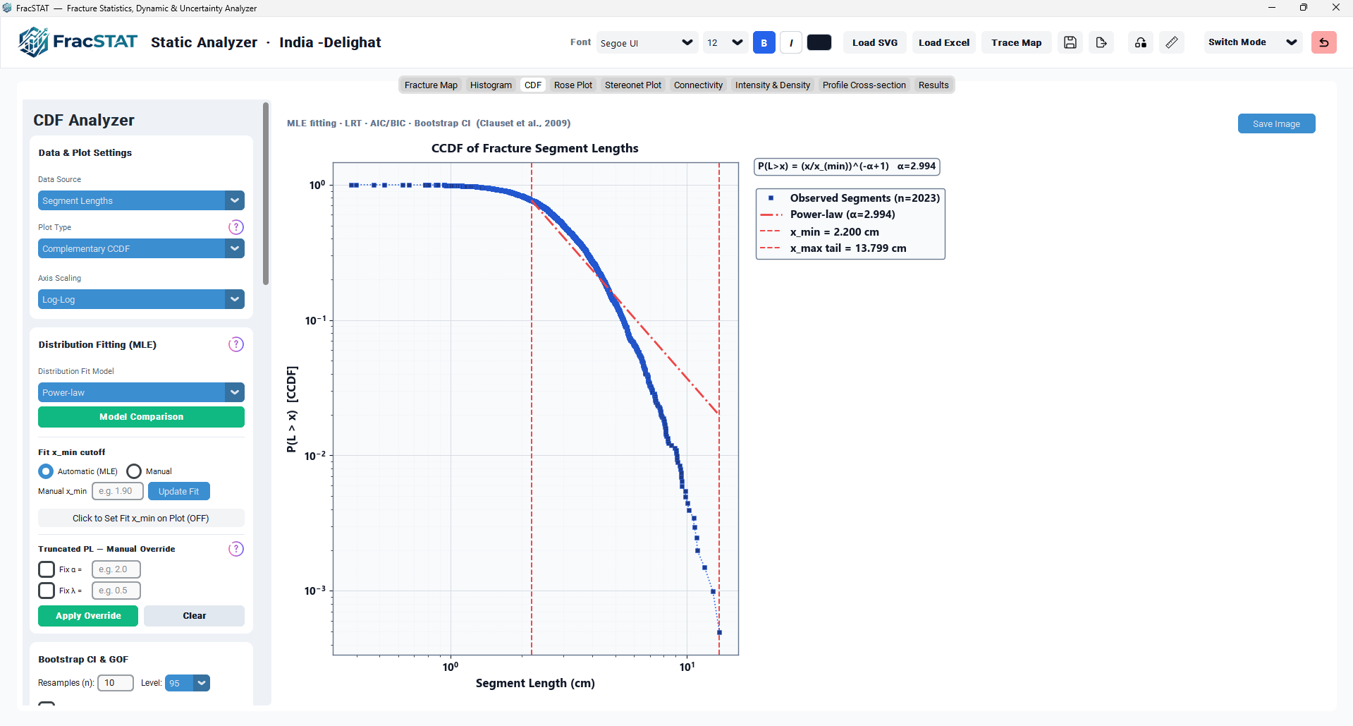
The CDF tab is arranged as a two‑column workspace: a scrollable settings sidebar (approximately 330 px wide) on the left, and a resizable plot canvas with an accompanying live statistics panel on the right. The statistics panel is docked at the bottom of the same sidebar column, below the settings cards, so that the numeric output of the currently selected model remains visible alongside the controls that produced it.
1.1 Sidebar Card Groups
The sidebar is organised into six functional cards, presented top‑to‑bottom in the order a user would typically configure an analysis: Data & Plot Settings, Distribution Fitting (MLE), Bootstrap CI & GOF, Plot Toggles, Appearance & Colors, and Axis Bounds & Canvas, followed by the live Statistics Summary panel.
| Card | Primary Function |
|---|---|
| Data & Plot Settings | Choose data source (segment vs. trace lengths), plot type, and axis scaling. |
| Distribution Fitting (MLE) | Select and configure the theoretical model(s) fitted to the tail of the distribution, including x_min cutoff mode and Truncated Power‑law manual overrides. |
| Bootstrap CI & GOF | Configure and trigger non‑parametric bootstrap resampling for parameter confidence intervals and a refit‑based goodness‑of‑fit p‑value. |
| Plot Toggles | Toggle auxiliary plot elements: x_min cutoff line, DKW confidence band, residuals subplot, on‑plot equation, and grid. |
| Appearance & Colors | Title, legend position, line/marker/grid/spine widths, point size, and a full colour palette for every plotted element and each of the five fit curves. |
| Axis Bounds & Canvas | Manual axis limits and explicit plot canvas pixel dimensions. |
| Statistics Summary | Scrollable, auto‑updating panel presenting descriptive statistics and, for the active fit model(s), all MLE parameters, information criteria, and goodness‑of‑fit diagnostics, plus the multi‑model comparison table when applicable. |
1.2 Toolbar
A slim toolbar sits above the plot canvas, displaying the caption "MLE fitting · LRT · AIC/BIC · Bootstrap CI (Clauset et al., 2009)" as a permanent reminder of the statistical framework in use, and a Save Image button that exports the current figure at the DPI configured in the application‑wide Settings page, including any floating legend or equation annotation that would otherwise be cropped.
1.3 Move Elements Mode
When the workspace‑wide "Move Elements" toggle is active, the on‑canvas legend and the on‑canvas equation annotation both become individually draggable. Their released positions are captured in axes‑fraction coordinates and are honoured on every subsequent redraw and by the Save Image export, so a legend repositioned to avoid overlapping a data cluster remains in that position until explicitly reset.
2. Data Input
2.1 Upstream Data Sources
The CDF tab does not load files directly; it consumes the results table already computed by the Static Analyzer for the currently loaded dataset, which arrives from one of three upstream pathways: SVG trace maps (vector fracture traces tessellated into straight segments and scaled into the calibrated real‑world profile box), spatial Excel/CSV tables (orientation tables carrying real X1/Y1/X2/Y2 endpoint coordinates), and legacy orientation‑only Excel/CSV tables (which may still supply a per‑row Length value even without spatial coordinates).
2.2 Data Source Selection
| Option | Underlying Column | Statistical Unit |
|---|---|---|
| Segment Lengths | Length_m (per straight segment) | Individual fracture segment |
| Trace Total Lengths | TraceLengthM (summed per trace) | Complete fracture trace |
Segment lengths are the finer‑grained population and are typically preferred for fractal/power‑law length‑scaling studies. Trace total lengths aggregate all segments belonging to one continuous fracture and are preferred when the object of study is the geological discontinuity rather than its digitisation artefacts.
2.3 Data Cleaning Applied Before Analysis
Before any statistic is computed, the raw column is sorted ascending and every non‑positive or non‑finite value is discarded. This guards against zero‑length degenerate segments (which can arise from duplicated vertices in a traced SVG) and against NaN values in trace aggregation. If, after this filtering, zero valid observations remain, the plot area displays an explanatory message rather than raising an error.
2.4 Minimum Sample Size for Fitting
Distribution fitting (the powerlaw MLE engine) is only attempted when the cleaned
sample contains more than 10 observations (n > 10). Below this threshold the module
still renders the empirical curve but does not attempt a theoretical fit, since MLE parameter
estimates for two‑parameter models are not meaningfully identifiable from very small samples.
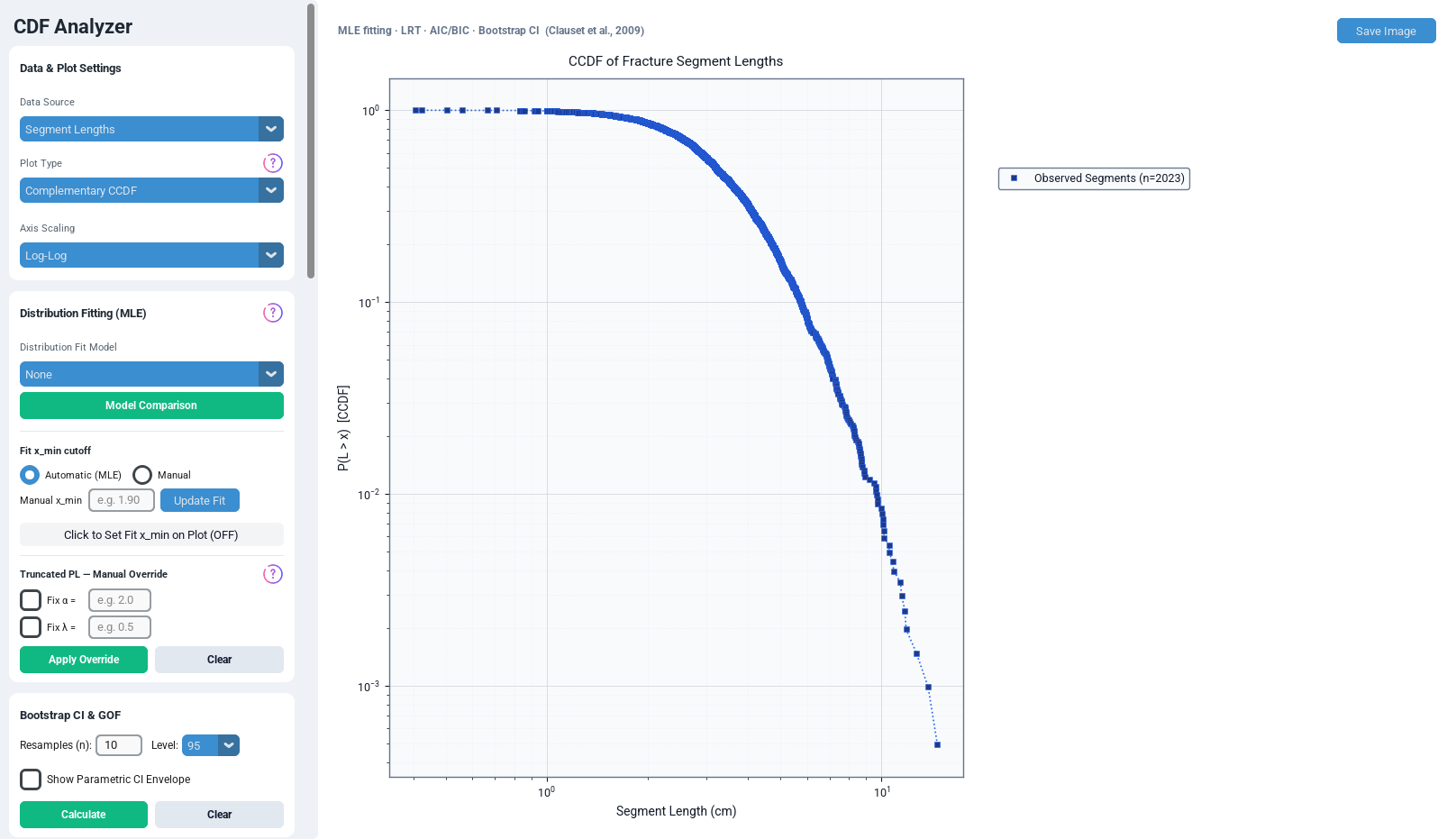
3. Settings and Controls, Card by Card
Unless stated otherwise, every control triggers an immediate redraw. Controls that would trigger an expensive maximum‑likelihood refit are explicitly flagged, since the module distinguishes style‑only redraws from heavy redraws for performance reasons (see Section 10).
3.1 Data & Plot Settings
| Control | Type | Options | Effect |
|---|---|---|---|
| Data Source | Dropdown | Segment Lengths; Trace Total Lengths | Selects the underlying length population. Triggers a full heavy redraw including MLE refit. |
| Plot Type | Dropdown | Cumulative Frequency; Cumulative CDF; Complementary CCDF; Q‑Q Plot; P‑P Plot | Chooses which empirical/theoretical comparison is rendered. |
| Axis Scaling | Dropdown | Log‑Log; Semi‑Log (X); Semi‑Log (Y); Linear | Controls the matplotlib axis transform applied to the main plot. Not applied to P‑P plots, which are always linear on [0,1]. |
3.2 Distribution Fitting (MLE)
| Control | Type | Effect |
|---|---|---|
| Distribution Fit Model | Dropdown | None; Power‑law; Exponential; Log‑normal; Weibull; Truncated Power‑law; Auto Best Fit. "Auto Best Fit" runs the full model‑selection procedure. |
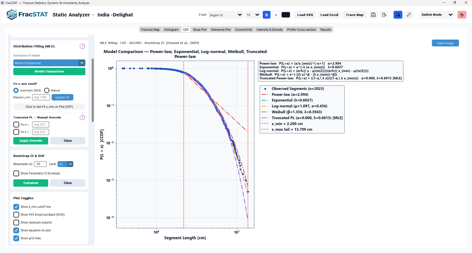
| Model Comparison | Button + dialog | Opens a dialog letting the user choose an arbitrary subset of models to compare side‑by‑side using AIC/BIC/KS/LRT machinery, without being constrained to the full five‑model panel. |
| Fit x_min cutoff — Automatic (MLE) | Radio button | The tail threshold x_min is estimated by the powerlaw library by scanning candidate cutoffs and minimising the KS distance between the empirical and fitted tail. |
| Fit x_min cutoff — Manual | Radio + entry + Update button | Fixes x_min to a user‑supplied value. Requires pressing Update Fit (or Enter) to apply and forces a fresh MLE refit. |
| Click to Set Fit x_min on Plot | Toggle button | Enters an interactive picking mode: the next mouse click on the plot reads the clicked x‑coordinate, writes it into the Manual x_min field, switches to Manual mode, and triggers a refit. |
| Truncated PL — Fix α = | Checkbox + entry | Locks the truncated‑power‑law scaling exponent to a user‑supplied value; the truncation rate λ is then re‑optimised for that fixed α. |
| Truncated PL — Fix λ = | Checkbox + entry | Locks the truncation rate; α is then re‑derived in closed form for that fixed λ. |
| Apply Override / Clear | Buttons | Apply Override recomputes the constrained truncated power‑law fit and its KS statistic; Clear removes both overrides and restores the ordinary two‑parameter MLE fit. |
3.3 Bootstrap CI & GOF
| Control | Type | Default | Effect |
|---|---|---|---|
| Resamples (n) | Numeric entry | 10 | Number of bootstrap resamples drawn (with replacement) for both the parameter confidence interval and the goodness‑of‑fit p‑value. Higher values tighten the interval at proportionally higher computation cost. |
| Level | Dropdown | 95% | Confidence level (90 / 95 / 99 %) used to compute the percentile bootstrap interval. |
| Show Parametric CI Envelope | Checkbox | Off | Overlays a shaded envelope on the CDF/CCDF curve spanning every combination of the bootstrap parameter confidence bounds (a conservative visual band, not itself a formal CI on the curve). Each bound curve is re‑conditioned at x_min by the same (F(x) − F(x_min)) / (1 − F(x_min)) identity used for the central fit (Section 4.9), so the envelope closes to zero width at the cutoff rather than fanning out from it. |
| Calculate | Button | — | Runs the bootstrap procedure for every model currently selected for plotting and caches the result. |
| Clear | Button | — | Disables bootstrapping and removes cached bootstrap results from the current redraw (the model fit itself is retained). |
3.4 Plot Toggles
| Control | Default | Effect |
|---|---|---|
| Show x_min cutoff line | On | Draws vertical dashed reference lines at the fitted x_min and at the maximum tail value, labelled with their numeric values. |
| Show 95% Empirical Band (DKW) | Off | Shades a Dvoretzky–Kiefer–Wolfowitz distribution‑free confidence band around the empirical CDF/CCDF curve. |
| Show residuals subplot | Off | Adds a secondary axes beneath the main CDF/CCDF plot showing standardised residuals between the empirical curve and each fitted model. |
| Show equation on plot | On | Draws the fitted model's closed‑form equation, with substituted parameter values, as a floating annotation on the canvas. |
| Show grid lines | On | Toggles major/minor gridlines on both axes. |
3.5 Appearance & Colors
| Control | Type | Purpose |
|---|---|---|
| Custom Title | Text entry | Overrides the automatically generated plot title (which otherwise states the plot type and sample count). |
| Legend Position | Dropdown | Outside Bottom, Outside Right, best, the four matplotlib corner anchors, center, or None. Persists a dragged legend anchor between redraws until changed. |
| Grid Width | Numeric entry | Line width, in points, of the major/minor gridlines. |
| Border Width | Numeric entry | Line width of the plot's outer spines. |
| Point Size | Numeric entry | Marker size (points) for observed‑data markers and for P‑P/Q‑Q scatter points; clamped to 0.5–40. |
| Outer Background / Plot Background / Grid Color / Border Color / CDF Line Color / Point Color | Colour swatch buttons | Full colour customisation of every non‑fit plot element, applied without re‑running the MLE fit. |
| Fit: Power‑law / Exponential / Log‑normal / Weibull / Truncated PL | Colour swatch buttons | Independent colour assignment for each of the five candidate model curves, consistent across the main plot, the residuals subplot, and the CI envelope. |
3.6 Axis Bounds & Canvas
| Control | Type | Effect |
|---|---|---|
| X min / X max / Y min / Y max | Numeric entries (blank = auto) | Overrides matplotlib's automatic axis limits on the corresponding axis. Only applied when both a lower and upper value are supplied and the lower value is smaller than the upper. |
| Reset Bounds to Auto | Button | Clears all four manual bound fields. |
| Plot Area Size — Width / Height (px) | Numeric entries | Rebuilds the matplotlib Figure and its Qt canvas at an explicit pixel size (default 700 × 850, a portrait‑leaning box matching the conventional aspect of published CDF/CCDF figures). |
| Reset Size to Auto | Button | Resets the Width/Height entry fields to 700 × 850 px. Note: the canvas rebuild triggered by this button currently reconstructs the figure at 1000 × 1000 px rather than the 700 × 850 px shown in the fields — a known discrepancy between the displayed defaults and the rebuilt canvas size. |
3.7 Statistics Summary Panel
This panel is not an input control but an always‑current, colour‑banded, scrollable read‑out of every statistic produced by the current configuration. It automatically re‑renders whenever the plot redraws, grouping values under bold section headers (e.g. "Descriptive", "Power‑law", "Auto Best Fit") and, for the Auto Best Fit and Model Comparison modes, embedding a horizontally scrollable results table directly in the sidebar in addition to the plot canvas.
3.8 Reset Defaults
A single Reset Defaults button at the foot of the sidebar restores every setting to its factory value, clears the MLE fit cache, and rebuilds the entire tab.
4. Mathematical Background
Let the cleaned, sorted sample of n positive fracture lengths be denoted L = {L₁ ≤ L₂ ≤ … ≤ Lₙ}. All formulas below use this notation; x refers to a length value on the horizontal axis.
4.1 Empirical Descriptive Statistics
The statistics panel always reports the following descriptive quantities, computed on the full cleaned sample independent of any theoretical fit:
| Statistic | Formula | Interpretation |
|---|---|---|
| n | count of L | Sample size |
| Min / Max | L₁, Lₙ | Range of observed lengths |
| Q1, Median, Q3 | 25th, 50th, 75th percentiles | Robust central tendency and spread |
| IQR | Q3 − Q1 | Interquartile range |
| Mean (μ̂) | (1/n) Σ Lᵢ | Arithmetic mean length |
| Std. Dev (s) | √[ (1/(n−1)) Σ (Lᵢ − μ̂)² ] | Sample standard deviation (Bessel‑corrected) |
| CV | s / μ̂ | Coefficient of variation (dimensionless spread) |
| Total Length | Σ Lᵢ | Cumulative fracture length in the sample |
| Skewness | Fisher–Pearson adjusted, requires n ≥ 8 | Asymmetry of the length distribution |
| Kurtosis | Adjusted excess kurtosis, requires n ≥ 8 | Tail heaviness relative to a normal distribution |
4.2 Empirical Cumulative Functions
For the sorted sample, rank rᵢ = n − i + 1 (i.e. Lᵢ is exceeded by n − i observations). Three empirical curves are available:
The Complementary CCDF is the conventional choice for fractal/scaling analysis because a true power‑law tail appears as a straight line on log–log axes, making deviations from linearity — and hence departures from pure scale‑invariance — visually apparent. Working with the complementary cumulative form rather than a binned histogram is also the recommended practice for heavy-tailed data, because it uses every observation and introduces no binning parameter (Clauset et al., 2009).
4.3 Power‑law Model
α is the scaling exponent. The theoretically interesting and frequently reported range for natural fracture networks is roughly 1.5 < α < 3.5 (Bonnet et al., 2001), and the exponent controls whether the network's connectivity and flow behaviour are dominated by the few longest fractures or by the many short ones (Bour and Davy, 1997).
Every survival function in this section is conditional on x ≥ x_min. Each model is fitted to the tail above x_min only, so the distribution being estimated — and the curve actually drawn — is the conditional one,
equivalently (F(x) − F(x_min)) / (1 − F(x_min)) for the CDF, which is what
powerlaw's cdf() methods return
(Clauset et al., 2009, §3.1;
Alstott et al., 2014). A correctly
conditioned model has F(x_min) = 0 by construction. Printing the
unconditional S(x) as the fitted equation misstates the annotation by the factor
1/S(x_min) — measured on synthetic tails, that error reached 62% for the exponential, 98.5%
for the log‑normal, and roughly 100% for the stretched exponential. The power‑law form above
happens to be already conditional as written, since (x/x_min)^(−α+1) equals 1 at x = x_min;
the other four need their normalising denominator shown explicitly, and do so below.
4.4 Exponential Model
λ (units of inverse length) is the decay rate; its reciprocal 1/λ is the characteristic length scale of the population. The x_min shift in the exponent is the conditioning: the unconditional e^(−λx) differs from it by the constant factor e^(−λ·x_min).
4.5 Log‑normal Model
μ and σ are the mean and standard deviation of ln(L). The log‑normal model is common where fracture length reflects the multiplicative combination of several independent growth processes. The ½ that appears in the textbook unconditional survival function is a special case of the denominator here: erfc[(ln x_min − μ)/(σ√2)] is the tail mass above x_min, and it equals 1 (giving the familiar ½ after the standard factor) only in the limit x_min → 0. Dividing by it is what normalises the plotted curve to 1 at x_min.
4.6 Weibull (Stretched‑Exponential) Model
β is the shape parameter (β = 1 recovers the exponential model) and λ is a scale parameter. FracSTAT labels this Weibull in the user interface because that is the more familiar name in geoscience and reliability contexts. The subtracted (λ·x_min)^β term is the conditioning supplied by powerlaw's conditional CDF and is not negligible at realistic x_min.
4.7 Truncated Power‑law Model
The density is a power law with an exponential cutoff, and its survival function is obtained by integrating that density from x to infinity — which yields an upper incomplete gamma function, not the density's own shape:
where Γ(s, z) is the upper incomplete gamma function (Aban et al., 2006, §2; Clauset et al., 2009, table 2.3). This model superimposes an exponential cutoff on a power‑law scaling regime and is frequently invoked when a genuinely scale‑invariant fracturing process is bounded by a finite physical control, such as mechanical layer thickness — the situation in which power-law scaling in real fracture populations is expected to break down at large lengths (Marrett et al., 1999).
α is used exactly as the library reports it. In powerlaw 2.0.0,
Truncated_Power_Law._pdf_base_function is
x**(-self.alpha) * exp(-self.Lambda * x) (distributions.py), so
fit.truncated_power_law.alpha is already the conventional pdf exponent α of
Clauset et al. (2009, table 2.3).
No ±1 conversion is applied or needed. Adding 1 "to convert" reports
every truncated‑power‑law exponent a full unit too steep: on synthetic tails drawn with
α = 2.500 / 3.000 / 1.800 the library recovers 2.542 / 2.977 / 1.822, and the +1 version would
print 3.542 / 3.977 / 2.822. Since α ≈ 2 is the boundary between a finite and an infinite
mean, a whole‑unit shift changes the geological reading of the result, not just its
decimals.
The module supports fixing either α or λ by the user, in which case the free parameter is re‑optimised by direct maximisation of the truncated‑power‑law log‑likelihood subject to the fixed value. In that override mode the plotted curve and the recomputed KS statistic both use the normalised conditional survival ∫ₓ∞ t^(−α) e^(−λt) dt ⁄ ∫x_min∞ t^(−α) e^(−λt) dt, evaluated by quadrature with the same α convention.
4.8 Maximum Likelihood Estimation and x_min Selection
All parameter estimates use maximum likelihood, not least‑squares curve fitting, following Clauset et al. (2009). When x_min is not fixed by the user, the library evaluates every candidate cutoff present in the data, fits each model's parameters by MLE above that cutoff, computes the KS distance between the fitted model and the empirical tail, and selects the cutoff that minimises this distance. This avoids the well‑known bias of fitting a power‑law to the entire dataset (including the non‑scaling small‑length population that dominates most natural fracture length distributions).
Choosing x_min from the data costs statistical power. The selected cutoff is itself an estimate, and discarding everything below it reduces the effective sample to ntail. Estimated exponents therefore carry more uncertainty than the printed digits imply, and the uncertainty in x_min propagates into α. The bootstrap (Section 5.4) is the mechanism for quantifying this, and Clauset et al. (2009, §3.3, §4) discuss both the KS-based selection rule and its cost. In fracture data specifically, the cutoff often has a physical interpretation — the resolution limit below which short traces were not mapped (Pickering et al., 1995) — and comparing the fitted x_min against the known mapping resolution is a useful sanity check.
4.9 Model‑Fit Anchoring for Display
Because the theoretical CDF/CCDF is normalised over [x_min, ∞) while the empirical curve is normalised over the full sample, the displayed theoretical curve is rescaled by a multiplicative anchor factor so that it passes exactly through the empirical curve's value at x_min. This anchoring preserves the shape and relative comparison of the tail fit while making the visual overlay directly comparable to the empirical curve across the full displayed range.
Anchoring is a display transform only — it moves the conditional curve of Section 4.3 onto the empirical scale; it does not make an unconditional formula correct. The two are separate steps and must not be conflated. The model curve fed to the anchor is always evaluated as
so that F_cond(x_min) = 0 and the survival is 1 at the cutoff before the anchor factor is applied. This is also the identity used by the bootstrap confidence‑band routine, which conditions each resampled model with the same expression rather than reusing the parent fit's scaling. A model that arrives at the anchor with F(x_min) ≠ 0 has not been conditioned and will show a visible offset at the left edge of the fitted range — that discrepancy is the diagnostic for the error, and it is why the equations in Sections 4.4–4.7 carry their x_min terms explicitly.
5. Algorithms
5.1 Empirical‑Curve Construction
- Extract the selected length column (segment or trace) from the current results table.
- Discard non‑finite and non‑positive values; sort the remainder ascending.
- Compute rank‑based frequency/CDF/CCDF arrays as defined in Section 4.2.
- Plot the requested representation, applying the chosen axis‑scaling transform.
5.2 MLE Fit‑and‑Cache Algorithm
Fitting is the most computationally expensive operation in the module, so the module maintains
an in‑memory cache keyed on a tuple of (hash of the cleaned data array, selected fit model,
active comparison‑model set, data source, x_min mode, manual x_min value). Before invoking
powerlaw, the cache is checked; on a hit, every downstream quantity (fitted
object, tail sample, log‑likelihoods, AIC/BIC, KS statistics) is restored without
recomputation. On a miss:
import io, warnings
from contextlib import redirect_stdout
import powerlaw

# Suppress console chatter from the powerlaw library
with redirect_stdout(io.StringIO()), warnings.catch_warnings():
    warnings.simplefilter("ignore")
    fit = powerlaw.Fit(tail_sample, xmin=x_min if manual_mode else None,
                       discrete=False, verbose=False)

# Extract tail sample (observations >= fitted x_min)
tail = data[data >= fit.xmin]
if len(tail) < 2:
    raise ValueError("Fewer than 2 points remain in the tail above x_min.")

# Compute per-model log-likelihoods, AIC, BIC, KS
for model_name in ALL_MODELS:
    dist = getattr(fit, model_name)
    ll   = dist.loglikelihoods(tail).sum()
    k    = MODEL_PARAMS[model_name]
    aic  = 2*k - 2*ll
    bic  = k * np.log(len(tail)) - 2*ll
    ks_stat, ks_p = stats.ks_1samp(tail, dist.cdf)
    cache[model_name] = dict(ll=ll, aic=aic, bic=bic, ks=ks_stat, ks_p=ks_p)
The cache evicts the oldest entry once more than three distinct configurations are stored — a small LRU‑style bound that keeps memory bounded while still covering rapid toggling between recently examined models.
5.3 Auto Best Fit / Model Comparison Selection
Given the AIC (or small‑sample‑corrected AICc when n_tail / k < 40), BIC, and KS rank of every candidate model, the algorithm proceeds as follows:
- Rank every model independently by AIC/AICc, by BIC, and by KS statistic; average the three ranks into a composite rank used for default ordering.
- Identify the AIC‑minimising model and the BIC‑minimising model separately.
- Declare a consensus model only if the AIC‑minimising and BIC‑minimising models coincide and are unique.
- Run every pairwise log‑likelihood‑ratio test between the consensus model and every other candidate via the library's
distribution_compareroutine. - Declare a single Preferred model only when AIC and BIC agree, the winner is within the top two by KS, no rival is indistinguishable (p ≥ 0.05), and no rival is significantly favoured (p < 0.05 with ratio favouring the rival).
- If any condition fails, report every model within ΔAIC/ΔAICc ≤ 2 or ΔBIC ≤ 2 of the leader as 'plausible', together with Akaike and BIC model‑averaging support weights, so the user sees the genuine ambiguity.
5.4 Bootstrap Resampling
Both procedures below are non-parametric and parametric bootstraps respectively, in the sense of Efron and Tibshirani (1993): the first resamples the observed tail to characterise parameter uncertainty, the second simulates from the fitted model to characterise the null distribution of the fit statistic.
5.4.1 Parameter Confidence Intervals
- Draw a resample of size equal to the tail sample, with replacement.
- Refit the selected model to the resample at the already‑established x_min (kept fixed to isolate parameter uncertainty from x_min‑selection uncertainty).
- Record the fitted parameter value(s).
- Repeat n_boot times; report the percentile interval at the requested confidence level for every parameter (Efron and Tibshirani, 1993, ch. 13).
Holding x_min fixed makes these intervals conditional. They describe the uncertainty in the parameters given that cutoff, and therefore understate total uncertainty, since x_min was itself estimated from the same data (Section 4.8). Percentile intervals are also the simplest of the bootstrap interval constructions and can be biased for skewed sampling distributions; bias-corrected alternatives are described by Efron and Tibshirani (1993, ch. 14). The practical response is to re-run the fit at two or three nearby cutoffs (Section 8.3) and confirm that the exponent is stable.
5.4.2 Parametric Bootstrap GOF p‑value
A conventional (asymptotic) KS p‑value assumes the theoretical CDF was specified in advance of seeing the data, which is not true here. The module therefore computes a refit‑based, simulation‑driven GOF p‑value, following the procedure of Clauset et al. (2009, §4): generate a synthetic dataset from the fitted model's own random‑number generator, refit from scratch, compute its KS statistic against its own refitted model, and repeat n_boot times. The reported p‑value is the fraction of simulated KS statistics that equal or exceed the KS statistic actually observed on the real data (with add‑one Laplace smoothing to avoid an impossible p = 0 from a finite simulation).
The p-value answers whether the data are consistent with the fitted model, and a large value is therefore weak evidence — it means the model cannot be ruled out, not that it is correct, and several of the five candidates may well be un-rejectable on the same sample (Clauset et al., 2009). The resolution of the p-value is also bounded by n_boot: with the default of 10 resamples the smallest distinguishable value is of order 0.1, which is why the limitation in Section 12 recommends raising it substantially before quoting a result.
5.5 Interactive x_min Picking
When mouse‑picking mode is enabled, the next left‑click registered inside the plot axes is intercepted: its data‑space x‑coordinate is written into the Manual x_min field (to four significant figures), the cutoff mode is switched to Manual, picking mode is deactivated, and a refit is triggered — giving the user an immediate, visual way to test how sensitive the fitted parameters are to the choice of tail cutoff.
6. Statistical Methods
6.1 Kolmogorov–Smirnov Goodness of Fit
| Quantity | Source | Interpretation |
|---|---|---|
| KS stat (powerlaw) | The powerlaw library's internal D statistic, used during x_min selection | Internal diagnostic consistent with the library's x_min search; primarily useful for comparing candidate x_min values against each other. |
| KS statistic (SciPy) | scipy.stats.ks_1samp against the fitted CDF (Virtanen et al., 2020) | Independently computed, standard one‑sample KS statistic (Massey, 1951); used as the basis for all AIC/BIC/LRT model ranking in this module. |
| KS p‑value (SciPy asymptotic) | scipy.stats.ks_1samp two‑sided p‑value | The classical asymptotic p‑value. Reported for reference but is descriptive only, since it does not account for x_min and parameter estimation from the same sample. |
| GOF p‑value (bootstrap, refit KS) | Section 5.4.2 parametric bootstrap | The statistically appropriate goodness‑of‑fit p‑value for an estimated model; requires the Bootstrap CI & GOF card to be run. |
6.2 Dvoretzky–Kiefer–Wolfowitz (DKW) Confidence Band
This distribution‑free band provides a simultaneous 95% confidence envelope around the empirical CDF/CCDF that is valid regardless of the true underlying distribution (Dvoretzky et al., 1956), making it a useful visual companion to (but not a substitute for) a specific model's parametric confidence interval. Because ε depends only on n, the band is a constant vertical width on the probability axis — which appears strongly asymmetric once plotted on logarithmic axes, and is correspondingly uninformative in the extreme tail where F̂ is itself close to 0 or 1.
6.3 Information Criteria
| Criterion | Formula | Notes |
|---|---|---|
| AIC | 2k − 2·ln(L) | k = number of free parameters (1 for power‑law/exponential, 2 for log‑normal/Weibull/truncated power‑law); L = maximised likelihood over the tail sample (Akaike, 1974). |
| AICc | AIC + 2k(k+1) / (n_tail − k − 1) | Small‑sample‑corrected AIC; used as the primary information criterion whenever n_tail / k_max < 40. |
| BIC | k·ln(n_tail) − 2·ln(L) | Penalises additional parameters more heavily than AIC as n_tail grows, favouring simpler models in larger samples (Schwarz, 1978). |
| Akaike / BIC weights | exp(−½Δᵢ) normalised over all candidates | Interpreted as the relative probability that model i is the Kullback–Leibler‑best (Akaike) or Bayes‑best (BIC) model among the candidate set. |
Every criterion here is relative, and only within this candidate set. A model can rank first on AICc while still fitting the data poorly; the ranking says which of the five candidates is least bad, not whether any of them is adequate. That question is answered by the goodness-of-fit test of Section 6.1, not by the information criteria (Clauset et al., 2009, §5). Comparisons are also valid only between models fitted to the same tail sample: because the likelihood is computed over observations above x_min, two fits with different x_min values have different ntail and their AIC/BIC values are not comparable.
6.4 Likelihood‑Ratio Test (LRT)
For any pair of candidate models, the log‑likelihood ratio R and its asymptotic significance p
are obtained from the powerlaw library's distribution_compare
routine (Alstott et al., 2014), which
implements the normalised likelihood-ratio test for non-nested models of
Vuong (1989) as applied to
heavy-tailed distributions by
Clauset et al. (2009, appendix C).
A positive R favours the first‑named model, a negative R favours the second; p <
0.05 is treated as a statistically significant preference, while p ≥ 0.05 is treated as the
two models being statistically indistinguishable — a result the module reports explicitly
rather than silently defaulting to whichever model happened to have the lower AIC.
7. Visualization & Figure Components
7.1 Plot Types
| Plot Type | Horizontal Axis | Vertical Axis | Typical Use |
|---|---|---|---|
| Cumulative Frequency | Length | Raw count of observations ≥ x | Absolute‑count view; not itself a probability. |
| Cumulative CDF | Length | P(L ≤ x), 0 → 1 | Standard cumulative distribution function. |
| Complementary CCDF | Length | P(L > x), 1 → 0 | Preferred for scale‑invariance / power‑law diagnosis on log–log axes. |
| Q‑Q Plot | Theoretical quantiles | Empirical quantiles | Compares the shape of the fitted model against the data in length units; departures from the 1:1 reference line indicate where the model over‑ or under‑predicts length. |
| P‑P Plot | Theoretical cumulative probability | Empirical cumulative probability | Compares the two distributions on a common [0,1] scale; more sensitive to disagreement in the bulk than the tails. |
7.2 Axis Scaling Options
Log‑Log scaling is the conventional choice for power‑law diagnosis (a straight line indicates scale‑invariant behaviour); Semi‑Log(X) and Semi‑Log(Y) are useful for isolating exponential behaviour (a straight line on Semi‑Log(Y) indicates an exponential tail); Linear scaling is most useful for small samples or for a plain, non‑technical presentation.
7.3 Residuals Subplot
When enabled, the standardised residual at each observed tail point is computed as the empirical minus the anchored theoretical curve value, divided by the standard deviation of the residuals across the tail. A well‑fitting model shows residuals scattered without systematic trend around zero, while a curved or trending residual pattern indicates the theoretical model captures the wrong functional shape even if its overall KS statistic appears acceptable.
7.4 On‑Plot Equation Annotation and Legend
The fitted model's closed‑form CDF/CCDF equation, with the estimated parameter values substituted in and any bootstrap confidence interval appended in square brackets, is rendered as a floating, draggable annotation box on the canvas, positioned by default just outside the top‑right of the axes. The legend lists every plotted series (observed data, each active model curve, x_min/x_max reference lines, the DKW band, and the CI envelope where enabled) and can be placed at any of the standard matplotlib anchor points or in one of two dedicated outside‑the‑axes positions designed to avoid ever overlapping the data.
7.5 Save Image
The Save Image toolbar button rasterises the current figure at the DPI configured in the application Settings page (default 300 dpi), including the floating legend and equation annotation via matplotlib's extra‑artists mechanism so that neither is cropped out of the saved file. Exported images are written into the project's dedicated plot‑exports folder, following the same naming and folder convention used by every other Static Analyzer plot tab.
8. Step‑by‑Step Example Workflows
8.1 Example 1 — Diagnosing Scale‑Invariant Behaviour
- Load an SVG fracture trace map (or a spatial Excel/CSV table) in the Static Analyzer and confirm the Fracture Map tab renders correctly.
- Open the CDF tab; leave Data Source at Segment Lengths and set Plot Type to Complementary CCDF with Axis Scaling set to Log‑Log.
- Set Distribution Fit Model to Auto Best Fit and inspect the Statistics Summary panel's "Final Recommendation" line.
- If a single Preferred model is reported with Power‑law or Truncated Power‑law as the winner, and the fitted α falls in the range typically reported for tectonic fracture networks (roughly 1.5–3.5), this is supportive (not conclusive) evidence of scale‑invariant fracturing across the sampled length range.
- Enable Bootstrap CI & GOF with 100–500 resamples to obtain a defensible confidence interval on α before quoting it in a report.
8.2 Example 2 — Comparing Segment vs. Trace Populations
Run the Auto Best Fit procedure once with Data Source set to Segment Lengths, and once with it set to Trace Total Lengths. A material difference in the preferred model or in x_min between the two runs indicates that the network's connectivity/segmentation (how many segments make up each trace) is itself influencing the apparent length‑scaling behaviour, which should be investigated alongside the Connectivity tab's I‑Y‑X node statistics before drawing conclusions from either population alone.
8.3 Example 3 — Testing Sensitivity to the Tail Cutoff
- With any single model selected, enable Click to Set Fit x_min on Plot and click at several different points along the empirical curve.
- Observe how the fitted parameter values, KS statistic, and AIC/BIC change as x_min moves — a fit whose parameters are stable across a wide range of x_min choices is considerably more defensible than one that changes sharply with small adjustments to the cutoff.
8.4 Example 4 — Truncated Power‑law with a Known Physical Boundary
- If independent evidence (e.g. measured bed thickness) suggests a specific truncation length scale, select Truncated Power‑law, check Fix λ =, enter the corresponding rate, and press Apply Override.
- Compare the resulting constrained fit's KS statistic and AIC against the unconstrained MLE truncated‑power‑law fit and against a plain power‑law fit, to test whether the proposed physical control is statistically consistent with the observed data.
9. Geological Interpretation
9.1 Power‑law (Fractal) Behaviour
A well‑supported power‑law fit across a wide length range is classically associated with self‑similar, scale‑invariant fracture growth, commonly attributed to fracture propagation and coalescence processes operating similarly at all observable scales (Bonnet et al., 2001). The exponent α controls how rapidly the population is dominated by short fractures versus how much cumulative length resides in the few longest fractures; low α values (closer to 1.5–2) indicate a length population with proportionally more very‑long fractures, which is significant for connectivity and percolation (Bour and Davy, 1997), and for the bulk permeability such a network can sustain (Odling, 1997).
A power-law fit over a limited range is not evidence of fractal geology. Observed scaling in fracture populations is bounded — below by mapping resolution and above by the size of the sampled area — and the range over which it can even be tested is usually only one to two orders of magnitude (Marrett et al., 1999). Over so narrow a range, several distributions are difficult to distinguish, which is why the likelihood-ratio comparison of Section 6.4 matters more than the visual straightness of the log–log plot (Clauset et al., 2009).
9.2 Exponential Behaviour
An exponential model implies a single characteristic length scale (1/λ), often interpreted as evidence of a single dominant mechanical control — such as fracture growth arrested by a specific bed thickness, an early joint set with a narrow length range, or a sampling/measurement artefact that truncates the population before scale‑invariance can develop.
9.3 Log‑normal Behaviour
A log‑normal fit is frequently interpreted as evidence that fracture length is the multiplicative product of several independent, comparably influential growth‑limiting factors, rather than a single dominant control — a pattern also common in populations affected by measurement/digitisation resolution limits at the short end of the range.
9.4 Truncated Power‑law Behaviour
A preferred truncated‑power‑law fit — scale‑invariant at short‑to‑intermediate lengths but decaying faster than a pure power‑law at the longest lengths — is the classic signature of scale‑invariant fracture growth that is ultimately bounded by a finite physical control, most often mechanical layer (bed) thickness in layer‑bound fracture systems. The fitted λ can, with care, be compared against independently measured layer thickness as a consistency check.
9.5 Practical Cautions for Interpretation
A statistically preferred model is a description of the sampled data, not proof of the underlying physical mechanism; multiple mechanisms can produce statistically similar length distributions. Truncation of the observed length range by outcrop or map extent (censoring) can masquerade as an exponential or truncated‑power‑law signature even when the true population is a pure power‑law; the Histogram tab's "Censor edge traces" option should be considered alongside this module when outcrop‑edge effects are suspected. Reported exponents and rates should always be accompanied by their bootstrap confidence intervals and by the model‑comparison evidence when used to support a specific geological or engineering conclusion.
10. Performance Optimization
10.1 MLE Fit Cache
Every completed MLE fit is cached keyed on the exact configuration that produced it, so switching back and forth between recently examined models, data sources, or x_min settings does not repeatedly pay the cost of a fresh non‑linear optimisation. The cache is deliberately small (three entries) to bound memory use while still covering the common "compare a couple of models" workflow.
10.2 Bootstrap Result Cache
Bootstrap confidence intervals and goodness‑of‑fit p‑values are the single most expensive computation the tab can perform (each resample requires a full model refit). Their results are cached separately from the MLE fit cache, keyed additionally on the resample count, confidence level, and the active model set, so that a redraw triggered by an unrelated cosmetic change reuses the previous bootstrap result rather than silently re‑running hundreds of refits.
10.3 Style‑only vs. Heavy Redraw Separation
Purely cosmetic changes (colour, legend, grid, axis bounds, point size) never touch either
cache or invoke powerlaw, keeping these adjustments instantaneous regardless of
dataset size or model complexity. Heavy redraws (data source, fit model, x_min cutoff, plot
type when it changes the fitted data) invalidate the fit cache where necessary and may re‑run
the full MLE and bootstrap pipeline.
10.4 Progress Reporting for Long‑Running Bootstraps
Rather than reporting progress on every single bootstrap iteration (which would itself impose UI‑repaint overhead on a large resample count), the progress callback throttles updates to roughly fifty reports across the full run for large n_boot values, while still reporting every iteration when n_boot is small enough that per‑iteration updates are cheap.
10.5 Warning Suppression
Several categories of benign, expected warnings emitted by the powerlaw and
SciPy optimisation internals (parameter estimates landing near an internal search‑bound edge,
or an internal initial guess falling outside declared bounds before the library's own clamping
resolves it) are filtered at the module level so they do not flood the console on every redraw
or bootstrap iteration, while genuinely actionable fit failures are still surfaced to the user
as an explicit pop‑up.
11. Advanced Features
11.1 Model Comparison Dialog
In addition to the automatic five‑model Auto Best Fit procedure, a Model Comparison dialog lets the user restrict the comparison to a hand‑picked subset of models (for example, comparing only Power‑law against Truncated Power‑law when the analyst already has a strong geological reason to exclude log‑normal and Weibull behaviour). The dialog offers Select All / Select None convenience buttons and runs the identical AIC/BIC/KS/LRT machinery, restricted to the chosen subset.
11.2 Truncated Power‑law Manual Override
Because MLE estimates for the two‑parameter truncated power‑law can occasionally land at the edge of the library's internal numerical search bounds for challenging datasets, the module allows either parameter (α or λ, or both) to be pinned to a user‑supplied, geologically motivated value. When only one parameter is fixed, the other is re‑derived analytically or by direct log‑likelihood maximisation over the tail sample so that the resulting curve remains a genuine (constrained) maximum‑likelihood fit rather than an arbitrary hand‑drawn line, and the KS statistic, log‑likelihood, AIC, and BIC are all recomputed consistently for the constrained model.
The α entered in the Fix α = field is the conventional pdf exponent of Section 4.7 — the exponent of x in p(x) ∝ x^(−α) e^(−λx) — which is also exactly what the library stores and what the annotation reports. There is no offset between the value typed in, the value optimised, and the value displayed, so a value taken from a published truncated‑power‑law fit can be entered directly.
11.3 Interactive x_min Picking
The "Click to Set Fit x_min on Plot" feature turns the fitting cutoff into a directly manipulable, visual parameter rather than a number the analyst must estimate by trial and error in the sidebar entry field (see Section 5.5 for the full algorithm).
11.4 Draggable Legend and Equation
Both the legend and the equation annotation participate in the workspace's shared Move Elements mode; their final dragged positions are captured in axes‑fraction coordinates on mouse release and are preserved across redraws and included in the Save Image export, so a publication‑ready layout, once arranged, does not have to be re‑arranged after every parameter change.
11.5 Manual Axis Bounds and Explicit Canvas Sizing
For preparing figures to a fixed physical size or aspect ratio (for example, matching a journal's column width), the Axis Bounds & Canvas card allows every axis limit and the canvas's own pixel dimensions to be set explicitly, overriding matplotlib's automatic choices while the underlying statistics remain unaffected.
11.6 Software Dependencies
| Library | Role in this Module |
|---|---|
powerlaw | Core MLE fitting engine for all five candidate distributions, x_min search, and pairwise log‑likelihood‑ratio comparison. |
SciPy | One‑sample KS testing, descriptive statistics (skewness/kurtosis), numerical optimisation for the Truncated Power‑law manual override, numerical integration of the constrained density, and the complementary error function used in the log‑normal survival function. |
NumPy | All array‑based numerical computation, percentile‑based bootstrap interval construction, and random resampling (Harris et al., 2020). |
Matplotlib | All plotting, including log/linear axis transforms, the residuals subplot, the draggable legend and equation annotation, and PNG export (Hunter, 2007). |
PySide6 (via ui_common.qtk) | Every sidebar control, the Model Comparison dialog, and the scrollable Statistics Summary panel. |
12. Limitations
| Limitation | Description |
|---|---|
| Asymptotic KS p‑value validity | The asymptotic SciPy KS p‑value is not statistically valid on its own once x_min and model parameters have been estimated from the same data. Only the bootstrap‑based GOF p‑value (Section 5.4.2) is methodologically appropriate, and it must be computed explicitly. |
| Default bootstrap resample count | The default of 10 resamples gives unstable confidence intervals and GOF p‑values, chosen for responsiveness during exploratory analysis. This should be increased substantially (200–1000) before any value is quoted in a final report. |
| Censoring not auto‑detected | Censoring caused by finite outcrop, map, or image extent is not automatically detected or corrected. Users working with edge‑truncated data should consult the Histogram tab's edge‑censoring option before drawing scaling conclusions. |
| Digitisation artefacts | The module assumes the supplied length column already reflects the desired physical population. It does not itself distinguish artefacts of digitisation (e.g. an SVG curve tessellated into many short straight segments) from genuinely short natural fractures; the Curve Step setting on the Fracture Map sidebar controls this trade‑off upstream. |
| Displayed equation is the conditional tail law | Every fitted equation annotation reports the survival function conditional on L ≥ x_min (Section 4.3), because that is the distribution estimated from the tail sample and the curve that is drawn. It must not be read as the unconditional law of the whole fracture population; converting between the two requires the tail fraction, which the module does not estimate. |
| Main‑thread bootstrapping | All fitting and bootstrap computation runs on the main UI thread rather than a background worker thread, since matplotlib's TkAgg backend is not safe to drive concurrently from a worker thread. Very large bootstrap runs will therefore block interaction with the rest of the application until they complete. |
13. References
Sources are listed alphabetically within each group. In-text citations throughout this page link to the corresponding entry below.
13.1 Heavy-Tailed Distributions and Model Selection
- Aban, I. B., Meerschaert, M. M., & Panorska, A. K. (2006). Parameter estimation for the truncated Pareto distribution. Journal of the American Statistical Association, 101(473), 270–277. https://doi.org/10.1198/016214505000000411
- Akaike, H. (1974). A new look at the statistical model identification. IEEE Transactions on Automatic Control, 19(6), 716–723. https://doi.org/10.1109/TAC.1974.1100705
- Clauset, A., Shalizi, C. R., & Newman, M. E. J. (2009). Power-law distributions in empirical data. SIAM Review, 51(4), 661–703. https://doi.org/10.1137/070710111
- Dvoretzky, A., Kiefer, J., & Wolfowitz, J. (1956). Asymptotic minimax character of the sample distribution function and of the classical multinomial estimator. The Annals of Mathematical Statistics, 27(3), 642–669. https://doi.org/10.1214/aoms/1177728174
- Efron, B., & Tibshirani, R. J. (1993). An Introduction to the Bootstrap. Chapman & Hall/CRC, New York. https://doi.org/10.1201/9780429246593
- Massey, F. J. (1951). The Kolmogorov–Smirnov test for goodness of fit. Journal of the American Statistical Association, 46(253), 68–78. https://doi.org/10.1080/01621459.1951.10500769
- Schwarz, G. (1978). Estimating the dimension of a model. The Annals of Statistics, 6(2), 461–464. https://doi.org/10.1214/aos/1176344136
- Vuong, Q. H. (1989). Likelihood ratio tests for model selection and non-nested hypotheses. Econometrica, 57(2), 307–333. https://doi.org/10.2307/1912557
13.2 Fracture Scaling and Sampling
- Bonnet, E., Bour, O., Odling, N. E., Davy, P., Main, I., Cowie, P., & Berkowitz, B. (2001). Scaling of fracture systems in geological media. Reviews of Geophysics, 39(3), 347–383. https://doi.org/10.1029/1999RG000074
- Bour, O., & Davy, P. (1997). Connectivity of random fault networks following a power law fault length distribution. Water Resources Research, 33(7), 1567–1583. https://doi.org/10.1029/96WR00433
- Marrett, R., Ortega, O. J., & Kelsey, C. M. (1999). Extent of power-law scaling for natural fractures in rock. Geology, 27(9), 799–802. https://doi.org/10.1130/0091-7613(1999)027<0799:EOPLSF>2.3.CO;2
- Odling, N. E. (1997). Scaling and connectivity of joint systems in sandstones from western Norway. Journal of Structural Geology, 19(10), 1257–1271. https://doi.org/10.1016/S0191-8141(97)00041-2
- Pickering, G., Bull, J. M., & Sanderson, D. J. (1995). Sampling power-law distributions. Tectonophysics, 248(1–2), 1–20. https://doi.org/10.1016/0040-1951(95)00030-Q
13.3 Software
- Alstott, J., Bullmore, E., & Plenz, D. (2014). powerlaw: A Python package for analysis of heavy-tailed distributions. PLoS ONE, 9(1), e85777. https://doi.org/10.1371/journal.pone.0085777
- Harris, C. R., Millman, K. J., van der Walt, S. J., Gommers, R., Virtanen, P., Cournapeau, D., … Oliphant, T. E. (2020). Array programming with NumPy. Nature, 585(7825), 357–362. https://doi.org/10.1038/s41586-020-2649-2
- Hunter, J. D. (2007). Matplotlib: A 2D graphics environment. Computing in Science & Engineering, 9(3), 90–95. https://doi.org/10.1109/MCSE.2007.55
- Virtanen, P., Gommers, R., Oliphant, T. E., Haberland, M., Reddy, T., Cournapeau, D., … van Mulbregt, P. (2020). SciPy 1.0: Fundamental algorithms for scientific computing in Python. Nature Methods, 17(3), 261–272. https://doi.org/10.1038/s41592-019-0686-2
Methods statement for the CDF tab. A caption or methods paragraph for a result exported from this tab should record:
Fracture length distribution fitted by maximum likelihood following
Clauset et al. (2009), using the
powerlaw package (Alstott
et al., 2014). State the fitted model, α (or the model's parameters), xmin
and whether it was fitted or fixed, ntail, the model-selection criterion used
(AICc/BIC and any likelihood-ratio comparison), the KS statistic, and the number of bootstrap
resamples behind any confidence interval or GOF p-value. Quote the bootstrap GOF
p-value rather than the asymptotic KS p-value
(Section 6.1), and note that reported equations are conditional on
L ≥ xmin (Section 4.3).