Static Rose Tab
Located at static_analyzer/tabs/static_rose_tab.py, the Rose Plot
tab (implemented as the mixin class StaticAnglesTab) renders an equal-area,
strike-frequency rose diagram — a polar histogram in which each fracture segment is binned by
its trend (strike) azimuth, and the resulting frequency, optionally weighted by segment length,
is displayed as a radially scaled petal. Rose diagrams have been a cornerstone visualisation in
structural geology for over a century, providing an immediate quantitative impression of
preferred fracture orientations, orientation clustering versus dispersion, and the presence of
multiple fracture sets. Within FracSTAT, the Rose Plot tab operates purely on the geometric
results table produced by the Fracture Map tab and performs no stress resolution, making it a
Static Analyzer (geometry-only) tool distinct from the stress-dependent Rose tab found in the
Dynamic Analyzer workspace.
On this page
- 1. Interface Overview
- 2. Data Input
- 3. Settings and Controls, Card by Card
- 4. Mathematical Background
- 5. Algorithms
- 6. Statistical Methods
- 7. Visualization & Figure Components
- 8. Step‑by‑Step Example Workflows
- 9. Geological Interpretation
- 10. Performance Optimization
- 11. Advanced Features
- 12. Limitations
- 13. References
1. Interface Overview
The Rose Plot tab uses a two-column layout: a fixed-width (290 px), vertically scrollable
settings sidebar on the left, and an expandable polar plot canvas on the right hosting a
Matplotlib polar Axes embedded via FigureCanvasTkAgg. The Figure is sized
9 × 7 inches at 100 DPI and hosts one polar Axes
(static_rose_ax) plus one dedicated colorbar Axes
(static_rose_cbar_ax), whose position and visibility are recomputed on every
redraw according to the selected colorbar placement.
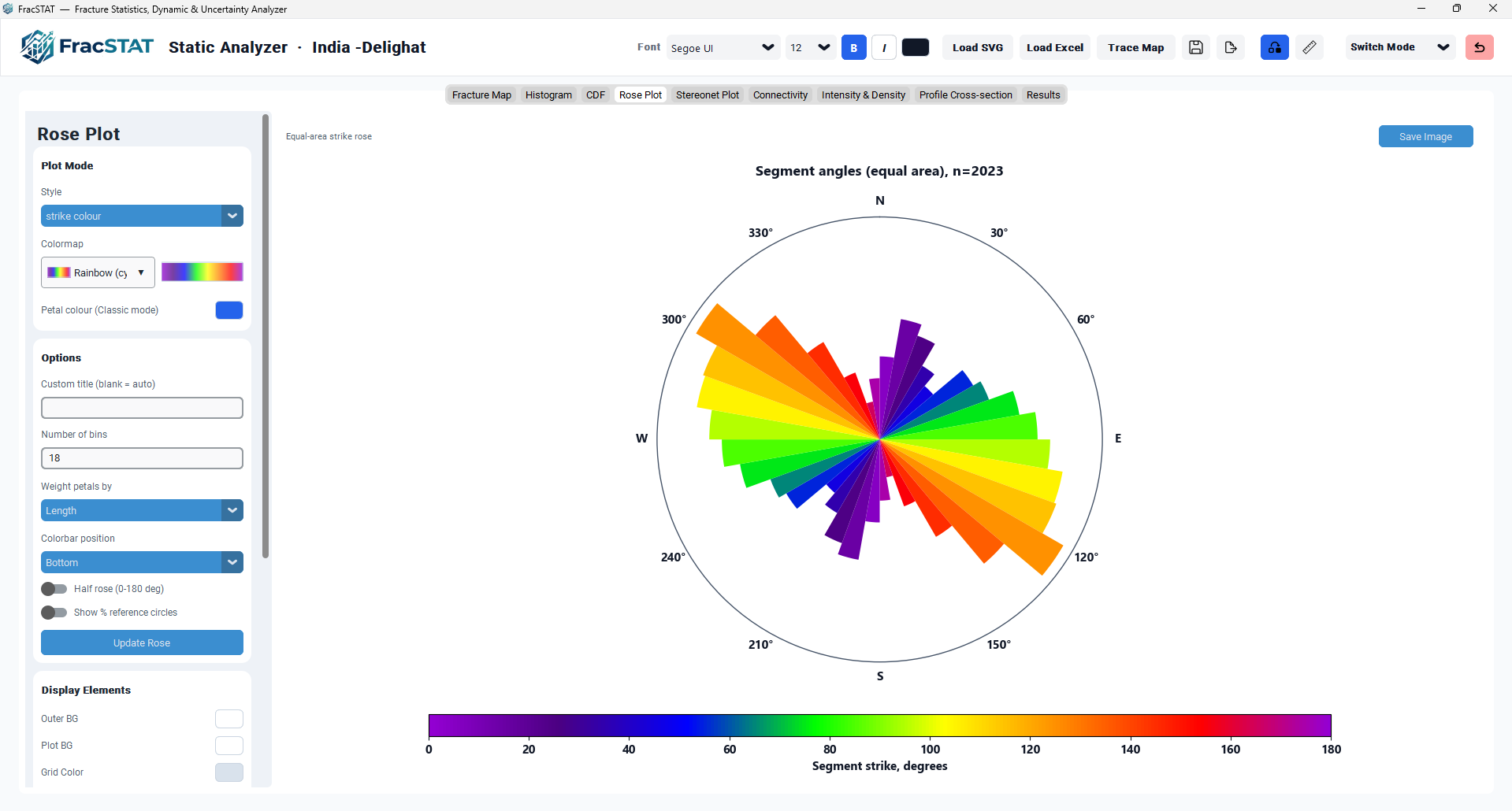
1.1 Sidebar Card Structure
| Card | Purpose | Key Widgets |
|---|---|---|
| Plot Mode | Selects the colouring scheme for the rose petals and, in Classic mode, the solid petal colour. | Style dropdown, Colormap dropdown + live preview swatch, Petal colour picker |
| Options | Controls the statistical construction of the diagram: binning, weighting, orientation range, and annotation of reference circles. | Custom title, Number of bins, Weight petals by, Colorbar position, Half rose switch, % reference circles switch, Update Rose button |
| Display Elements | Controls cosmetic rendering of plot background, grid, cardinal labelling, and plot boundary. | Outer BG / Plot BG / Grid Color pickers, Show grid lines / Show cardinal labels / Show N-S-E-W crosshairs checkboxes, Border Color picker, Border Width entry |
| Statistics | Read-only summary of the currently plotted dataset. | Segments, Mean Strike, Dominant Bin, Total Length labels |
1.2 Plot Canvas and Toolbar
A slim toolbar sits above the polar plot canvas, displaying the descriptive caption
"Equal-area strike rose" and a Save Image button. Clicking Save
Image invokes the shared save_plot_image() routine common to every Static
Analyzer tab, writing a timestamped PNG to the project's
FracSTAT_plot_exports/<project_slug> folder at the DPI configured in the
application-wide Settings page (default 300 DPI), with a confirmation dialog showing the
full output path.
2. Data Input
2.1 Upstream Data Sources
The Rose Plot tab does not implement its own file-loading logic. It reads directly from
self.results, the shared results DataFrame maintained by the Static Analyzer
workspace, which is refreshed whenever the user loads a new SVG fracture-trace file, a new
Excel/CSV orientation table, or changes the profile calibration. The tab automatically reflects
any such change without requiring user interaction through the workspace's
refresh_all_tabs() chain.
2.2 Required Columns
| Column | Type | Role in Rose Plot |
|---|---|---|
StrikeDeg | float, degrees, 0–360 (fully directed) | Source orientation value; folded to the 0–180° axial convention via strikes % 180.0 before binning. |
Length_m | float, project display units | Optional per-segment length used as the histogram weight when "Weight petals by" is set to Length. |
If StrikeDeg is absent, the tab shows an explanatory empty-state message on the
polar Axes. If StrikeDeg is present but every value is non-finite after validity
filtering, a separate "No valid strike angles found" message is shown. Both conditions are
handled gracefully without exceptions.
2.3 Compatible Upstream Data Sources
All four upstream data formats supported by the Static Analyzer flow into the Rose Plot tab.
SVG fracture-trace maps supply strike computed geometrically from the digitised trace endpoints,
corrected for the Y-axis-from-North azimuth. Excel/CSV segment-coordinate tables carry
pre-computed StrikeDeg values through unchanged. Legacy fracture-plane tables
(ID, Strike, Dip) supply Strike directly, with the optional Length column honoured for length
weighting. Trend/Plunge pole tables are converted internally to an equivalent Strike/Dip pair
before reaching the Rose Plot tab.
StrikeDeg is stored as a fully-directed 0°–360°
azimuth throughout the rest of the application (to preserve dip-direction information needed by
the Stereonet and Dynamic Analyzer tabs), the Rose Plot module performs its own modulo-180°
folding at draw time rather than relying on a pre-folded column.
3. Settings and Controls, Card by Card
Unless stated otherwise, every control triggers an immediate redraw through
_draw_static_rose(). Numeric entry fields commit on both the
Enter keypress and loss of focus (FocusOut), matching the convention
used throughout FracSTAT's Static Analyzer sidebars.
3.1 Plot Mode Card
| Control | Default | Description |
|---|---|---|
| Style | strike colour | Chooses between two rendering modes: strike colour (FracSTAT mode — petals coloured by bin midpoint via a colormap) and Classic (solid colour) (all petals in a single user-selected colour). The selected mode dispatches to either _draw_fracSTAT_rose() or _draw_classic_rose(). |
| Colormap | Viridis | Selects the Matplotlib colormap used in FracSTAT mode. A live 104×28 px gradient swatch is redrawn on selection. The resolved Matplotlib identifier is cached in static_rose_cmap_resolved to avoid repeated lookups on every redraw. |
| Petal colour (Classic mode) | #2563EB | Hex colour applied to every petal when Style is Classic. Exposed via the shared _StaticColorButton swatch/hex-entry widget. |
3.2 Options Card
| Control | Default | Valid Range | Effect |
|---|---|---|---|
| Custom title | "" (blank) | Free text | Overrides the auto-generated plot title (e.g. "Segment angles (equal area), n=…"). Leave blank to use the automatic title. |
| Number of bins | 18 | Integer, clamped [4, 180] | Number of equal-width azimuth classes spanning 0°–180°. Directly controls the angular resolution of the histogram. Out-of-range values are silently clamped and written back. |
| Weight petals by | Length | Length | Count | Whether each fracture contributes its measured Length_m (Length) or a uniform weight of 1 (Count) to its bin. For rows with missing or non-positive Length_m, a fallback weight of 1.0 is substituted. |
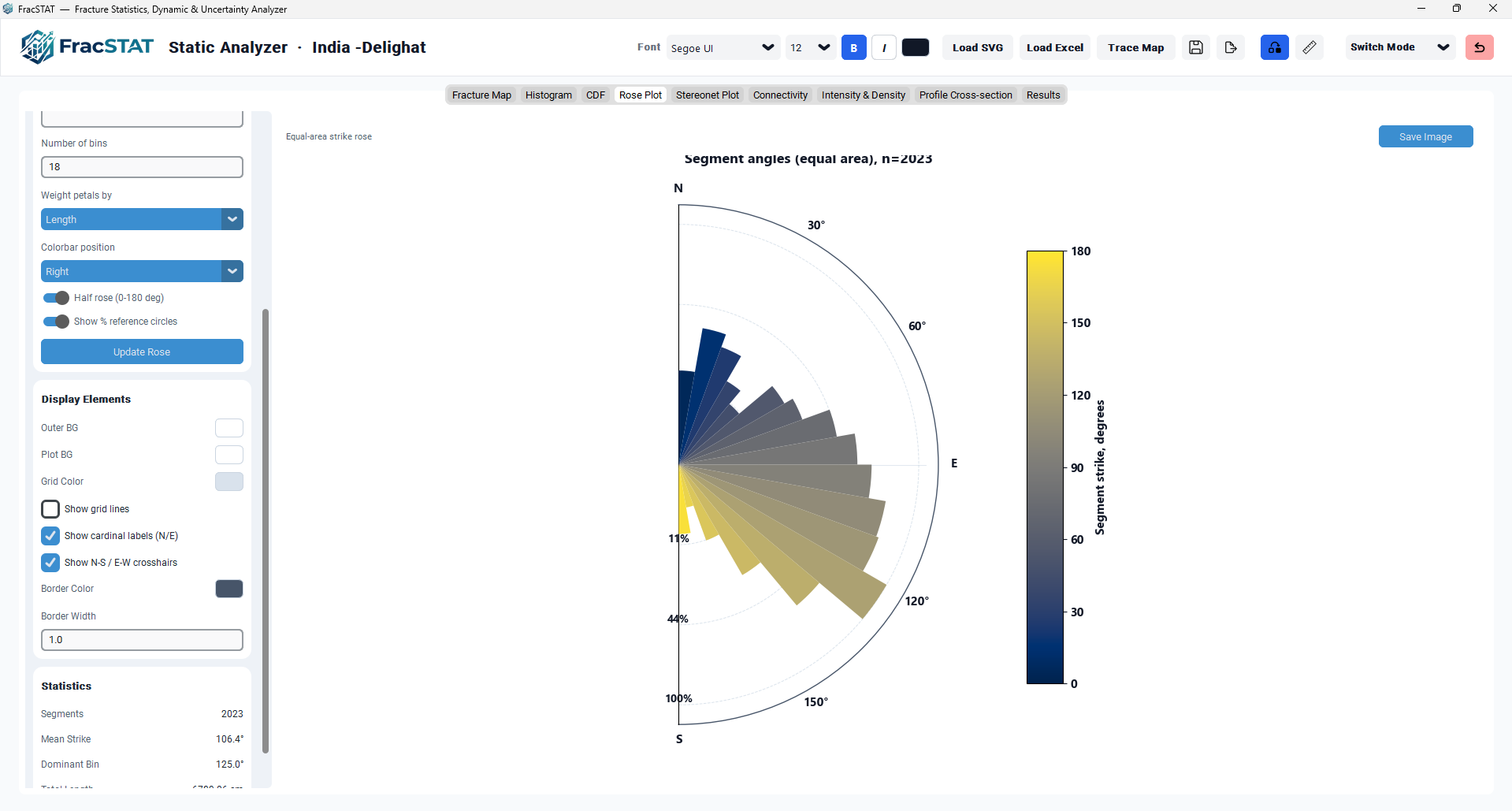
| Colorbar position | Bottom | Bottom | Top | Left | Right | None | Repositions or hides the colour-scale legend and adjusts the polar Axes bounding box to prevent overlap. Ignored in Classic mode. |
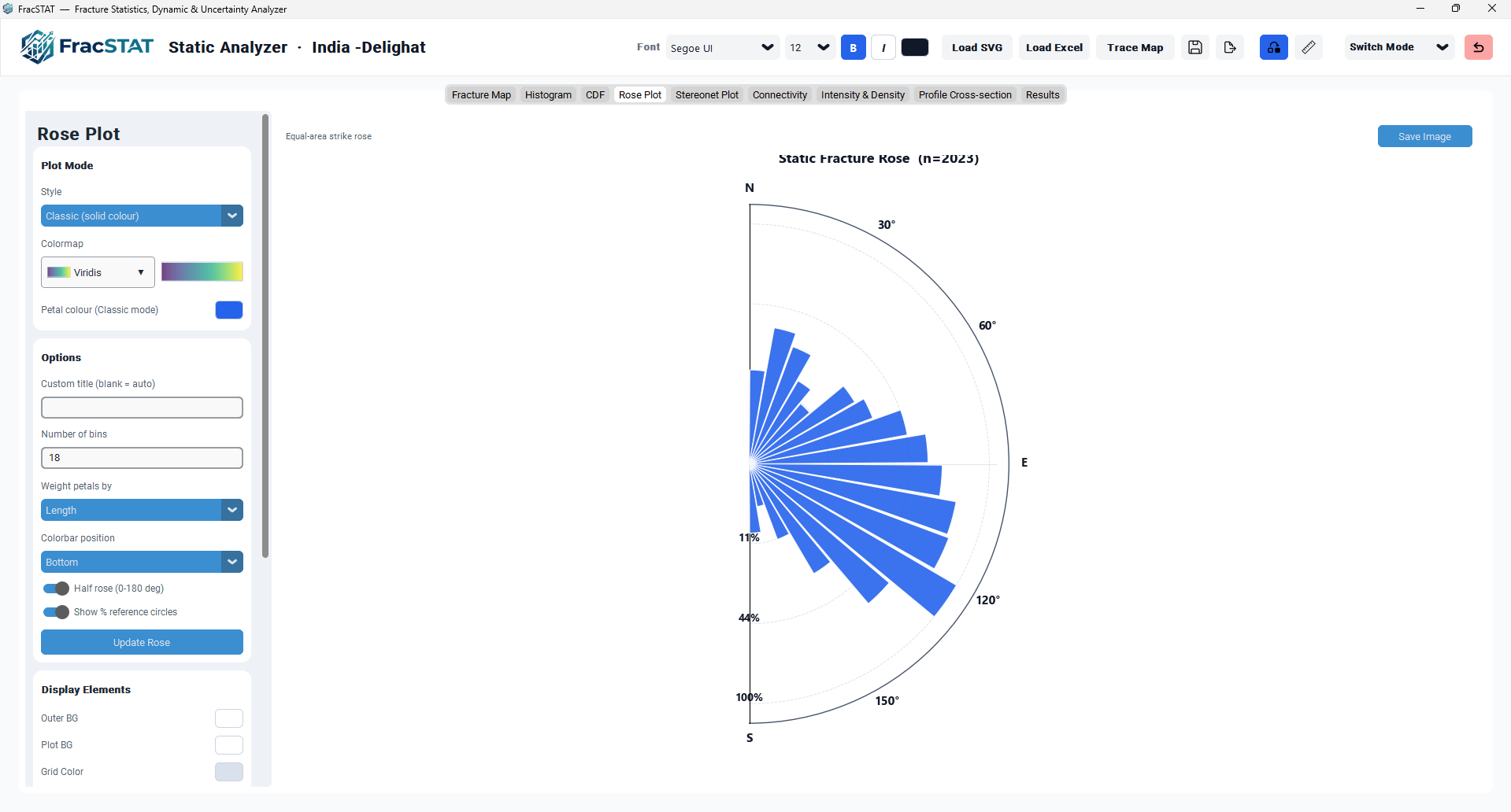
| Half rose (0–180° only) | Off | Boolean | When enabled, restricts the diagram to a semicircle spanning 0°–180°. When disabled, the histogram is mirrored into the 180°–360° half for the conventional full-circle axial rose. |
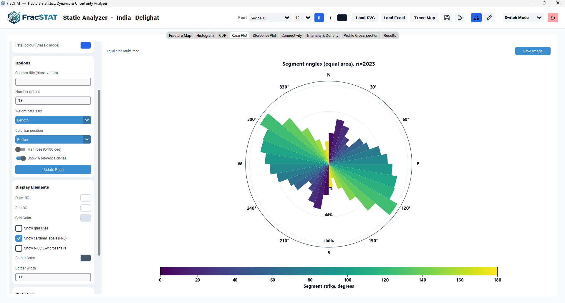
| Show % reference circles | Off | Boolean | Overlays three dashed concentric circles annotated with percentage-of-maximum labels calibrated to the equal-area (square-root) radius transform. See Section 4.5. |
| Update Rose (button) | — | — | Manually forces a redraw; provided for consistency even though most controls already redraw automatically. |
3.3 Display Elements Card
| Control | Default | Effect |
|---|---|---|
| Outer BG | #FFFFFF | Figure (outer canvas) background colour. |
| Plot BG | #FFFFFF | Polar Axes (inner plot) background colour. |
| Grid Color | #D9E2EC | Colour of the radial/angular grid lines when enabled. |
| Show grid lines | Off | Toggles the Matplotlib polar grid. |
| Show cardinal labels (N/E) | On | Replaces the 0°/90°/180°/270° angular tick labels with N/E/S/W; all other ticks remain numeric. |
| Show N-S / E-W crosshairs | Off | Draws faint radial spokes at the cardinal directions from the origin to 1.03 × the maximum petal radius. |
| Border Color | #475569 | Colour of the polar spine (outer plot boundary circle). |
| Border Width | 1.0 | Line width, in points, of the polar spine. |
3.4 Statistics Card (Read-Only)
The Statistics card is a read-only panel, recomputed on every redraw by
_rose_update_stats() from the raw, unbinned observations — not from the
discretised histogram — so its values are independent of the chosen Number of bins.
| Field | Description |
|---|---|
| Segments | Count of valid (finite) strike observations included in the diagram after data validation. This is the n value shown in the auto-generated title. |
| Mean Strike | The weighted axial (circular) mean strike in degrees, computed via the doubled-angle method in _static_axial_mean() (see Section 6.1). |
| Dominant Bin | The midpoint azimuth of the histogram bin carrying the greatest weighted frequency. Sensitive to the chosen bin count. |
| Total Length | Sum of Length_m across all valid segments in the project's active display unit. |
4. Mathematical Background
4.1 Axial (Bidirectional) Orientation Data
Fracture strike is an axial quantity: a fracture trending 040° is geometrically identical to one trending 220°, since both describe the same line in the horizontal plane. Axial data of this kind are 180°-periodic and cannot be treated with ordinary linear statistics (Mardia and Jupp, 2000). The Rose Plot module respects this by folding every strike value into the half-open interval [0°, 180°) prior to any statistical operation:
This folding is applied identically in both the FracSTAT-mode and Classic-mode drawing routines and is a prerequisite for the axial circular-mean formula in Section 6.1.
4.2 Weighting Scheme
Each observation i contributes a weight wi to its assigned azimuth bin. Two modes are supported:
where Li is the segment's real-world length (Length_m). When
length weighting is requested but Length_m is missing, non-finite, or non-positive
for a given row, a fallback weight of 1.0 is substituted for that row rather than discarding it.
Length weighting is the recommended default for fracture-trace data, because an unweighted count
of traces gives equal influence to a metre-scale joint and to a basin-scale fault and therefore
describes the sampling process at least as much as the fracture fabric itself
(Sanderson and Peacock, 2020).
4.3 Histogram Binning
Given B bins (clamped to [4, 180]), the bin edges form a uniform partition of the 0°–180° axial domain:
Each observation's folded strike is assigned to exactly one bin via NumPy's weighted histogram (Harris et al., 2020), producing bin totals and midpoints:
The class interval is a genuinely free parameter of the method rather than a cosmetic setting: too few bins smooth out real modes, while too many produce spurious spikes that reflect sampling noise (Wells, 2000). The 10° interval implied by the default B = 18 follows long-standing practice for two-dimensional geological orientation data (Curray, 1956), but it is advisable to inspect two or three bin counts before selecting the figure to publish.
4.4 Equal-Area (Square-Root) Radius Transform
A properly constructed rose diagram requires that the visual area of each petal — not its radial length — be proportional to the quantity it represents. Because the area of a circular sector scales with the square of its radius, FracSTAT computes the plotted radius as the square root of the weighted bin total:
This equal-area convention prevents bins with high raw frequency from visually dominating the diagram disproportionately, and ensures that comparisons of petal area between diagrams are quantitatively meaningful. The argument for the square-root radius was set out explicitly by Nemec (1988), who showed that a linear-radius rose exaggerates the dominant class because the reader's eye integrates sector area rather than sector radius; the same conclusion is reached from a perceptual standpoint by Wells (2000) and is recommended as standard practice by Sanderson and Peacock (2020). FracSTAT applies the transform unconditionally, in both plot modes, so no combination of settings can produce a linear-radius (area-distorting) rose.
4.5 Full-Circle Mirroring
Because strike is axial, a complete rose diagram must display the same frequency distribution twice — once in the 0°–180° half and once, by reflection, in the 180°–360° half. When Half rose is unchecked, the module concatenates bin midpoints and radii with a 180° angular offset:
This produces a visually symmetric diagram about the origin, matching the long-established convention for axial rose diagrams in the structural-geology literature (Curray, 1956). Note that the mirrored half contains no information that is not already in the first half; it is a display convention, and the choice between the full circle and the half rose of Section 3.2 is therefore purely presentational (see the discussion of rose-diagram conventions in Sanderson and Peacock, 2020).
4.6 Colour Mapping (FracSTAT Mode)
In strike colour mode, each petal is coloured according to its bin midpoint using a fixed linear normalisation over the full axial domain, independent of the actual data range:
Using a fixed 0°–180° normalisation (rather than normalising to the observed min/max strike) ensures the same azimuth is always rendered in the same colour across different datasets and sessions — important when visually comparing rose diagrams from multiple outcrops or wells.
4.7 Percentage Reference Circles
When enabled, three dashed reference circles are drawn at radii that are simple fractions of the maximum plotted radius rmax:
Because the plotted radius already embeds the square-root equal-area transform, the fraction of the maximum bin value represented by each circle is the square of the radial fraction:
The three default circles are therefore labelled approximately 11%, 44%, and 100% of the peak weighted bin value, giving a calibrated visual scale for judging petal size without reading exact numbers from an axis. Providing such a scale addresses a specific and frequently made criticism of published rose diagrams — that they are drawn without any indication of the magnitude the petals represent, and so cannot be read quantitatively (Sanderson and Peacock, 2020). Enabling this option, and reporting n in the title, is recommended for any rose diagram intended for publication.
5. Algorithms
5.1 Mode Dispatch
The top-level redraw entry point _draw_static_rose() is a two-way dispatcher
that inspects static_rose_mode_var and routes to one of two independent drawing
algorithms. If the Style string begins with "Classic", control passes to
_draw_classic_rose(); otherwise it passes to _draw_fracSTAT_rose().
Both routines share an identical outer skeleton — clear axes, validate data, compute the
weighted histogram, apply the equal-area transform, render petals, format the polar grid, set
the title, configure the colorbar, update the statistics panel, and request a canvas redraw —
but differ in how petal colour is derived.
5.2 FracSTAT-Mode Rendering Algorithm
| Step | Operation |
|---|---|
| 1 | Clear the polar Axes and colorbar Axes; apply outer/inner background colours. |
| 2 | Validate self.results is non-empty and contains StrikeDeg; otherwise show an empty-state message and abort. |
| 3 | Fold strikes to [0°, 180°) via modulo 180; discard non-finite values; abort with a message if none remain. |
| 4 | Resolve weights from Length_m (with 1.0 fallback for invalid entries) or uniform 1.0, depending on "Weight petals by". |
| 5 | Compute bin count B (clamped [4, 180]); build B+1 uniform edges over [0°, 180°); compute weighted histogram values[] and bin midpoints. |
| 6 | Abort with an empty-state message if the histogram sum is zero. |
| 7 | Resolve the active Matplotlib colormap; map every bin midpoint through a fixed Normalize(0, 180) to obtain one RGBA colour per bin. |
| 8 | If Half rose is enabled, use bins as-is; otherwise mirror bins, weights, and colours into the 180°–360° half. |
| 9 | Apply the equal-area square-root transform; draw all petals in one ax.bar() call with per-petal colour array and zero petal gap (full angular width). |
| 10 | Apply shared polar-grid formatting via _format_polar_grid. |
| 11 | Set the plot title (custom or auto-generated "Segment angles (equal area), n=…"). |
| 12 | Build a ScalarMappable from the same colormap/normalisation and delegate colorbar placement to _setup_rose_colorbar(). |
| 13 | Compute and push Segments / Mean Strike / Dominant Bin / Total Length into the Statistics card via _rose_update_stats(). |
| 14 | Request an idle canvas redraw via draw_idle(). |
5.3 Classic-Mode Rendering Algorithm
The Classic-mode algorithm mirrors steps 1–6 and 8–14 of the table above exactly, but omits
the colormap resolution and per-bin colour-array step. Every petal is rendered with the single
solid colour held in static_rose_color_var, a 90% opacity, and a petal angular
width of 0.92 × the full bin width to leave a visible gap between adjacent petals
— a more traditional discretised rose-diagram appearance. Because Classic mode carries no
data-dependent colour mapping, the colorbar Axes is always suppressed regardless of the
selected Colorbar position, and the polar Axes expands to fill the reclaimed space.
5.4 Shared Polar Grid Formatting
| Step | Operation |
|---|---|
| 1 | Fix the polar orientation convention: 0° at geographic North (set_theta_zero_location("N")), angles increasing clockwise (set_theta_direction(-1)) — the standard geological azimuth convention. |
| 2 | If Half rose is active, restrict the visible angular sector to [0°, 180°] via set_thetamin/thetamax. |
| 3 | Generate angular tick positions every 30°; substitute N/E/S/W labels at 0°/90°/180°/270° when cardinal labels are enabled. |
| 4 | Hide radial tick labels (petal length is read qualitatively or via the optional percentage circles). |
| 5 | Style the polar spine using Border Color and Border Width settings. |
| 6 | If crosshairs are enabled, draw faint radial spokes at the cardinal directions from the origin to 1.03 × the maximum petal radius. |
| 7 | Apply or suppress the angular/radial grid according to Show grid lines. |
| 8 | If % reference circles are enabled, delegate to the module-level helper _pct_reference_circles(). |
5.5 Colorbar Placement Algorithm
Given the selected Colorbar position, _setup_rose_colorbar() computes two
rectangles in Figure-fraction coordinates: one for the colorbar Axes and one for the
repositioned polar Axes, so that the polar plot never overlaps the legend. Horizontal
placements (Bottom/Top) receive tick marks every 20°; vertical placements (Left/Right) receive
tick marks every 30°, reflecting the differing available label space. Selecting "None", or
being in Classic mode, hides the colorbar Axes entirely and expands the polar Axes to an
enlarged default footprint.
def _pct_reference_circles(ax, max_r, palette, n_circles=3):
    """Draw dashed percentage reference circles on a polar axis."""
    if max_r <= 0:
        return
    theta_ring = np.linspace(0, 2 * np.pi, 361)
    for k in range(1, n_circles + 1):
        r_k = max_r * k / n_circles
        pct = int(round(100.0 * (k / n_circles) ** 2))
        ax.plot(theta_ring, np.full_like(theta_ring, r_k),
                color=palette["spine"], linewidth=0.7, linestyle="--",
                zorder=1, alpha=0.55)
        ax.text(np.deg2rad(180), r_k, f"{pct}%",
                color=palette["muted"], fontsize=8,
                ha="center", va="bottom", zorder=2)
Module-level helper function _pct_reference_circles() defined at module scope outside the class, so it requires no instance state and remains independently testable.
6. Statistical Methods
6.1 Weighted Axial (Circular) Mean
Ordinary arithmetic averaging is invalid for orientation data because of wrap-around
discontinuities — for example, the arithmetic mean of 179° and 1° is 90°, which is
geometrically nonsensical for near-parallel fractures straddling the 0°/180° boundary.
The correct treatment is to average the observations as unit vectors and take the direction of
the resultant (Fisher, 1993). For
axial (180°-periodic) data such as strike, the standard device is to double each angle before
forming the resultant and halve the result afterwards — the doubling transform of
Mardia and Jupp (2000, §2.3.2),
introduced for two-dimensional geological orientation data by
Krumbein (1939) and
Curray (1956). FracSTAT implements
exactly this in _static_axial_mean(strikes, weights):
Doubling each angle maps the 180°-periodic axial domain onto the standard 360°-periodic circular domain, where conventional vector-resultant averaging is valid; halving the resultant direction maps the answer back onto the physically meaningful 0°–180° range. The mean is always computed from the raw, unbinned observations — not the discretised histogram — so its value is independent of the chosen Number of bins. The same weights wi defined in Section 4.2 are used, so the reported mean is a length-weighted mean whenever length weighting is active.
6.2 Dominant Bin
The dominant (modal) orientation is reported as the midpoint of whichever histogram bin
carries the largest weighted total: argmax_k(V_k). Unlike the axial mean, this
statistic is sensitive to the chosen bin count and edge alignment, and should be interpreted
as a discretised estimate of the peak of the underlying orientation distribution rather than
an exact value. Its resolution is bounded below by the class interval itself, 180°/B
— 10° at the default setting — and for a peak that straddles a bin boundary the reported value
can jump by one full interval in response to a change of a single bin
(Wells, 2000). Where a
bin-independent estimate of the modal orientation is required, a kernel-density or
parametric-distribution approach on the unbinned angles is appropriate
(Fisher, 1993, §2.4); neither is
implemented in this tab.
6.3 Summary of Reported Statistics
| Statistic | Formula / Method | Sensitive to Bin Count? | Sensitive to Weighting Mode? |
|---|---|---|---|
| Segments (n) | Count of finite StrikeDeg values | No | No |
| Mean Strike | Doubled-angle weighted circular mean (§6.1) | No | Yes |
| Dominant Bin | argmax of weighted histogram | Yes | Yes |
| Total Length | Σ Length_m over all segments | No | No |
Total Length is computed over every row of the results table, including rows whose strike was discarded as non-finite, so it reports the total mapped trace length of the dataset rather than the sum of the plotted weights. It is therefore not equal to ΣVk in general, and does not change with the weighting mode.
7. Visualization & Figure Components
7.1 Polar Petal Bars
Petals are rendered with a single vectorised ax.bar() call in polar coordinates.
Bar centre angles equal the (possibly mirrored) bin midpoints in radians; bar heights equal
the equal-area radii rk; bar bottoms are fixed at zero. In FracSTAT mode
the bar width equals the full bin angular width so adjacent petals visually abut one another
(as in a continuous histogram). In Classic mode a 0.92 width factor introduces a visible
inter-petal gap for a more traditional, discretised rose-diagram appearance.
7.2 Colour Legend / Colour Bar
In FracSTAT mode, a ScalarMappable sharing the same colormap and fixed
0°–180° Normalize instance used for the petals is passed to Matplotlib's
fig.colorbar(), producing a legend labelled "Segment strike, degrees". Its
position (Bottom / Top / Left / Right / None) is fully reconfigurable, and the polar Axes'
bounding box is recomputed on every change to avoid overlap. The colour bar is intentionally
omitted in Classic mode, since a single solid petal colour carries no scale to legend.
7.3 Cardinal and Angular Labelling
Angular tick marks are placed every 30° around the full or half circle. When cardinal labelling is enabled, the four principal directions are rendered as N / E / S / W in place of 0° / 90° / 180° / 270°, while all remaining ticks continue to show numeric degree values — a hybrid convention familiar from paper-based structural fabric diagrams.
7.4 Reference Circles and Crosshairs
Two independent optional overlays aid quantitative reading of the diagram: the percentage reference circles (Section 4.7), which calibrate petal size against the peak bin value, and the N-S/E-W crosshair spokes, which provide a lightweight visual reference grid without the density of a full polar grid. Both can be enabled or disabled independently via their respective checkboxes in the Options card.
7.5 Empty-State Handling
Three distinct conditions each trigger a dedicated styled empty-state message rendered
directly on the polar Axes via _static_rose_empty_state(), rather than an
uncaught exception or a blank canvas: no data loaded / StrikeDeg column absent
("Load SVG or Excel fracture data"); all strike values non-finite ("No valid strike angles
found"); histogram sum is zero, for example all weights filtered out ("No plottable rose
values"). In all three cases the Statistics card fields are reset to a placeholder dash.
8. Step-by-Step Example Workflows
8.1 Example 1 — Quick-Look Orientation Screening
- Load an SVG trace map (or Excel/CSV) via the workspace header's Load SVG or Load Excel button; the Fracture Map, Rose Plot, and all other tabs populate automatically.
- Open the Rose Plot tab. With default settings (18 bins, Length weighting, FracSTAT strike-colour mode, full circle) the diagram immediately reveals one or more dominant petal directions.
- Read the Statistics card: Mean Strike gives the length-weighted average trend; Dominant Bin gives the single most frequent azimuth class, useful for checking whether the mean is being pulled between two conjugate sets.
- Toggle Show % reference circles to gauge, at a glance, what fraction of the dominant petal's weighted length the secondary petals represent.
8.2 Example 2 — Comparing Count-Based and Length-Weighted Fabrics
Switching Weight petals by from Length to Count on the same loaded dataset can reveal a different dominant orientation. Count weighting treats every fracture equally regardless of length; Length weighting emphasises the orientations carrying the greatest total trace length. Running both modes and comparing the resulting Dominant Bin and Mean Strike values is a standard diagnostic for distinguishing "many small" versus "few large" fracture populations — a meaningful distinction for flow-model permeability anisotropy inputs (Odling, 1997). Because fracture length distributions in rock are typically heavy-tailed, often approximately power-law (Bonnet et al., 2001), a small number of long traces can carry a large fraction of the total length, and the two weighting modes can legitimately identify different dominant sets in the same dataset.
8.3 Example 3 — Publication-Quality Figure Preparation
The steps below assemble a figure that carries the information a reader needs in order to interpret it — sample size, class interval, weighting mode, and a magnitude scale — which is what distinguishes a usable rose diagram from a decorative one (Sanderson and Peacock, 2020; Rougier et al., 2014).
- Set Colorbar position to "Bottom" and choose a colour-blind-friendly colormap such as Viridis or Cividis (see Section 4.6).
- Disable Show grid lines for a cleaner appearance, but enable Show cardinal labels and Show % reference circles for quantitative legibility.
- Enter a descriptive Custom title (e.g., "Joint set orientations, Outcrop A, n = 214"). Note that a custom title replaces the automatic one, which is where n would otherwise appear — so include n in the text you type.
- Increase Border Width slightly (e.g., to 1.4) for improved visibility at reduced print size.
- State the bin count and the weighting mode in the figure caption; neither is rendered on the plot itself.
- Click Save Image to export a high-resolution PNG to the project's plot-exports folder.
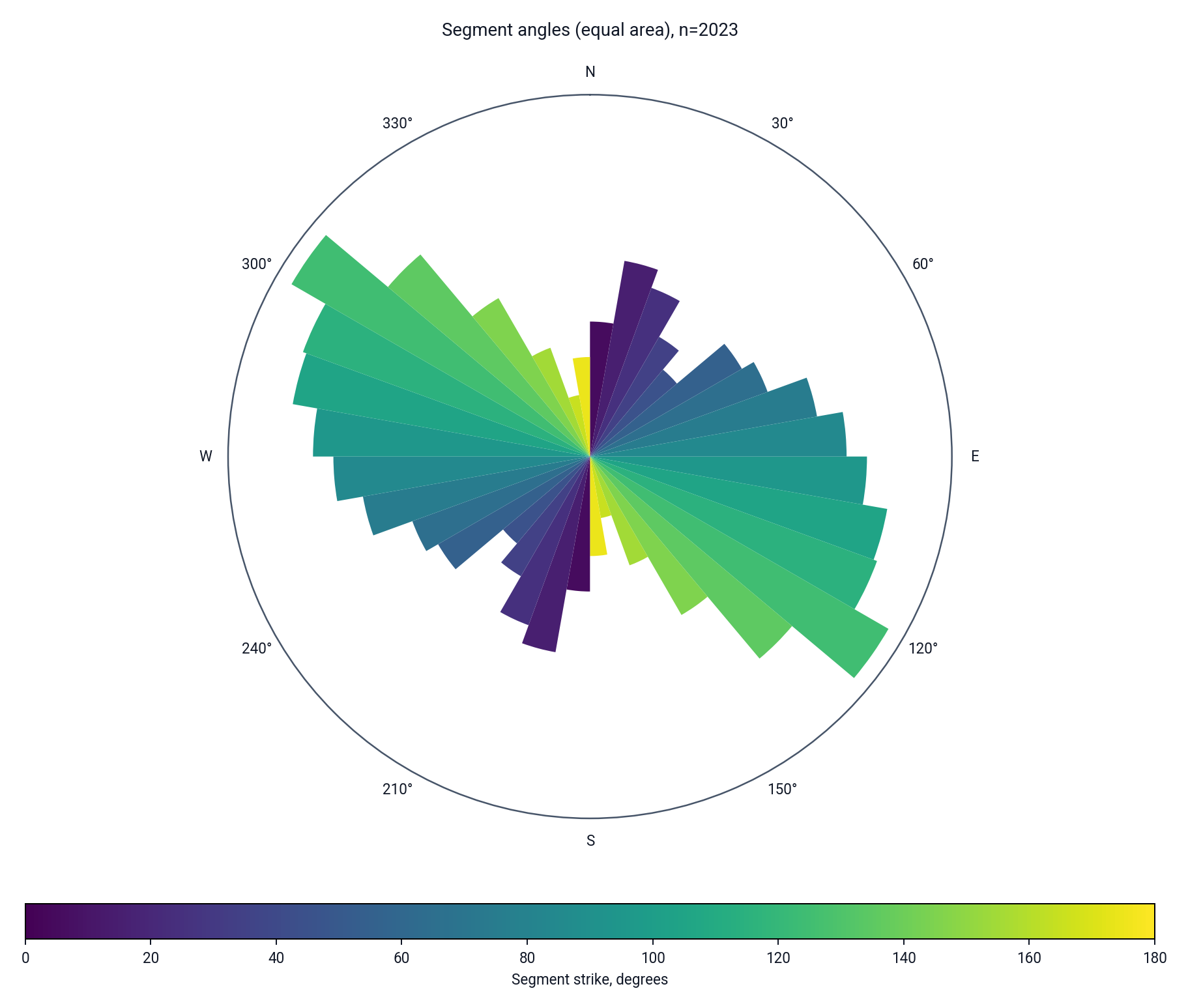
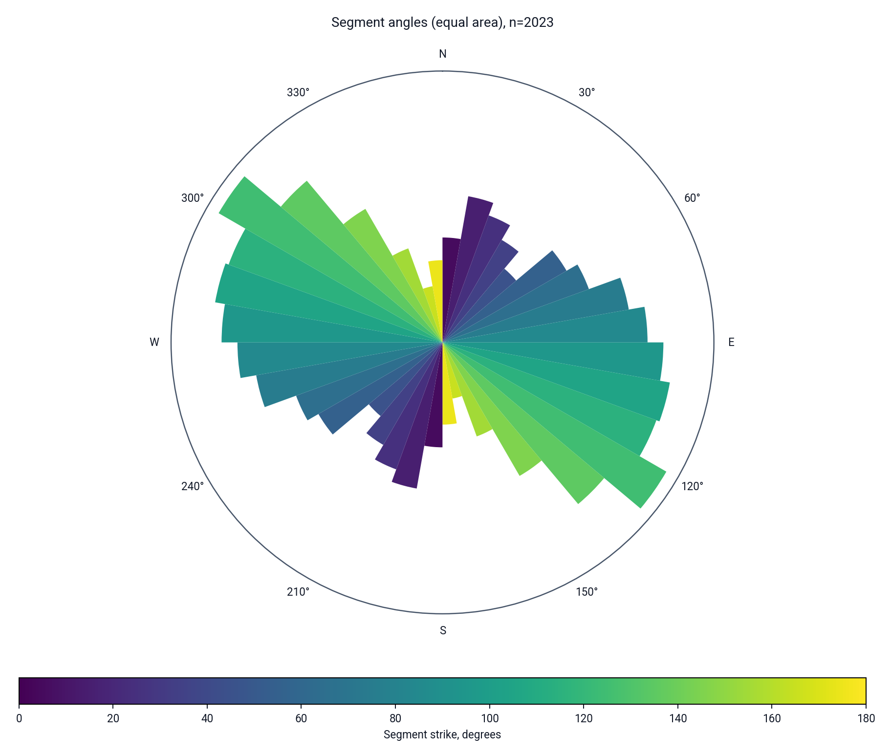
9. Geological Interpretation
9.1 Reading a Rose Diagram
A single sharply peaked petal (or symmetric petal pair in the full-circle presentation) indicates a strongly unimodal fracture fabric, consistent with a single dominant regional stress orientation acting during fracture formation — such as joints formed perpendicular to a uniaxial extension direction or systematic joints related to a single tectonic episode. Two petals separated by an acute angle (commonly 40°–70°) are the classic signature of a conjugate shear-fracture pair, and their angular bisector approximates the orientation of the maximum principal compressive stress (σ₁) at the time of formation (Anderson, 1951), following the Andersonian/Coulomb faulting framework used in FracSTAT's Dynamic Analyzer. Multiple broadly distributed petals of comparable magnitude suggest a polymodal or polyphase fracture history.
9.2 Significance of Length Weighting
Length-weighted rose diagrams better represent the orientation distribution of throughgoing, hydraulically or mechanically significant fractures, since long fractures typically dominate bulk rock-mass permeability and mechanical anisotropy (Odling, 1997). Count-based diagrams better represent the orientation distribution of fracture initiation events and can be more sensitive to sampling bias toward short, easily digitised features. The two diagrams together provide a complementary picture of the fracture population, and reporting both is recommended practice (Sanderson and Peacock, 2020).
9.3 The Mean Strike as a Design Parameter
The reported Mean Strike is frequently used as an input for downstream engineering workflows — for example, orienting a horizontal wellbore trajectory to intersect the dominant fracture set at a favourable angle for stimulation, or orienting a slope-stability kinematic analysis with respect to the governing discontinuity set (Priest, 1993). Because the statistic uses the doubled-angle axial-mean method, it remains geometrically valid even when the underlying distribution straddles the 0°/180° boundary — a common pitfall when analysts instead average raw azimuths arithmetically (Mardia and Jupp, 2000). It remains a summary of a single mode, however, and the caution in Section 6.1 applies before the value is carried into a design calculation.
9.4 Caution Regarding Sampling Bias
As with any orientation-frequency analysis derived from a two-dimensional trace map or outcrop pavement, the rose diagram is subject to orientation sampling bias: fractures whose strike is sub-parallel to a linear exposure, scanline, or window edge are systematically under-sampled relative to fractures oriented perpendicular to it. The standard correction is the weighting scheme of Terzaghi (1965), in which each observation is weighted by the reciprocal of the sine of the angle between the fracture and the sampling line or surface; censoring of long traces at the boundaries of a finite window biases length-weighted diagrams in addition (Priest and Hudson, 1981; Mauldon, 1998).
10. Performance Optimization
10.1 Vectorised Histogram and Colour Computation
All per-observation operations — modulo folding, weight resolution, and the weighted histogram
itself — are performed with NumPy array operations (np.histogram, boolean
masking, np.where) rather than per-row Python loops
(Harris et al., 2020), giving
effectively linear-time performance in the number of fracture segments, which routinely numbers
in the thousands to tens of thousands for digitised trace maps.
10.2 Colormap Resolution Caching
Resolving a user-facing colormap display name (e.g. "Red-Yellow-Blue") to its underlying
Matplotlib identifier ("RdYlBu") is performed once inside _on_rose_cmap_change()
and the result is cached in the instance attribute static_rose_cmap_resolved.
Subsequent redraws triggered by unrelated setting changes read the cached identifier directly
rather than re-resolving the dropdown's display string on every frame.
10.3 Idle-Draw Scheduling
The canvas is repainted via FigureCanvasTkAgg.draw_idle() rather than the
blocking draw(), deferring pixel-level rendering to the next Qt idle cycle.
This keeps rapid successive setting changes (e.g. dragging through bin-count values or
a fast sequence of colour-picker changes) from stalling the UI thread with redundant full
redraws.
10.4 Shared Geometry Computation
Because the Rose Plot tab performs no independent geometry recomputation — it consumes the DataFrame already computed once by the Fracture Map tab's geometry engine — reloading data or changing the profile scale triggers only a single shared O(n) geometry pass, not a duplicated per-tab recalculation. The Rose Plot tab's own per-redraw cost is limited to the histogram, colour-mapping, and rendering steps.
11. Advanced Features
11.1 Colormap Library
The Colormap dropdown draws from the same 25-entry, application-wide colour-scale catalogue used throughout FracSTAT, spanning perceptually uniform scientific colormaps (Viridis, Plasma, Inferno, Magma, Cividis), classic scales (Turbo, Jet, Parula — a bundled MATLAB-style approximation), diverging scales (Coolwarm, Spectral, Red-Yellow-Blue), cyclic scales (HSV, Twilight, Rainbow (cyclic)) well suited to angular data, and several thematic/sequential scales (Hot, Ocean, Terrain, Earth, and others). For the reasons set out in Section 4.6, the perceptually uniform and cyclic families are preferable for quantitative figures, and the classic non-uniform rainbow scales are best reserved for exploratory work (Crameri et al., 2020).
11.2 Half-Circle vs Full-Circle Presentation
The Half rose toggle allows analysts to choose between the compact 0°–180° semicircular presentation (useful when screen or print space is limited, or when comparing several diagrams side-by-side) and the traditional full-circle mirrored presentation expected in most published structural-geology figures. Both modes use identical statistical inputs; only the angular display range and the mirroring of bins differ.
11.3 Dynamic Colorbar Repositioning
Selecting a new Colorbar position does not merely relocate the legend graphic; the polar Axes'
own position rectangle is simultaneously recalculated via _setup_rose_colorbar()
so that the two never overlap and the plot remains centred and appropriately sized —
Bottom/Top placements reserve a horizontal strip and shrink the plot's vertical extent, while
Left/Right placements reserve a vertical strip and shrink its horizontal extent.
11.4 No "Reset to Defaults" Button
Unlike the Dynamic Analyzer's Rose tab, the Static Rose tab does not provide a "Reset to Defaults" button. To restore a control to its factory value, set it manually using the defaults listed in the tables of Section 3.
11.5 Relationship to the Dynamic Analyzer's Rose Tab
A structurally analogous but functionally distinct Rose tab exists in the Dynamic Analyzer
workspace (dynamic_rose_tab.py). That implementation supports colouring petals by
a resolved stress attribute (slip tendency, dilation tendency, fracture susceptibility, or
critical-stress state) rather than by strike itself, and additionally supports overlaying the
σ₁ azimuth as a reference line. Those attributes derive from resolving a stress tensor onto each
fracture plane, in the slip- and dilation-tendency framework of
Morris et al. (1996) and
Ferrill et al. (1999). The two
modules share the equal-area square-root radius convention and the general polar-histogram
construction, but the Static Rose tab documented here performs no stress resolution and requires
no stress-tensor input.
12. Limitations
| Limitation | Description |
|---|---|
| Dominant bin sensitivity | The Dominant Bin statistic is a discretised estimate dependent on the chosen Number of bins and on the fixed bin-edge alignment starting at 0°. It is not a continuous-distribution mode estimate (e.g. from kernel density estimation) and can shift between adjacent bins for small changes in bin count on noisy or sparse datasets (Wells, 2000). |
| No orientation-bias correction | Petal magnitudes are raw sampled totals. The Terzaghi (1965) weighting for fractures sub-parallel to the exposure or scanline, and length-bias corrections for traces censored at a window boundary, are not applied (Terzaghi, 1965; Priest and Hudson, 1981). See Section 9.4. |
| No dispersion or significance measure | No circular standard deviation, resultant length, confidence interval on the mean strike, or test against a uniform distribution is computed, so the diagram cannot indicate whether an apparent preferred orientation is statistically distinguishable from a random fabric (Mardia and Jupp, 2000, ch. 6). |
| Mean strike assumes unimodality | A single resultant direction is reported regardless of the shape of the distribution; for bimodal or polymodal fabrics it falls between the modes and is not physically meaningful (Section 6.1). |
| Fixed bin origin | Bin edges always begin at exactly 0°. A mode centred on a bin boundary is split between two adjacent petals, and there is no option to offset the bin origin to test the stability of the apparent modes. |
| Two-dimensional projection only | Only strike is used; dip is ignored entirely. Two fracture sets with identical strike but very different dip are indistinguishable on this diagram, and a rose diagram of strike alone cannot represent a three-dimensional fracture fabric. Use the Stereonet tab for full orientation analysis (Priest, 1993). |
| Segment-level, not fracture-level | The histogram is built from the segments present in the results table. Where a single curved or polyline fracture trace is stored as multiple segments, it contributes multiple observations, so count weighting reflects segmentation of the digitised geometry as much as the number of fractures. Length weighting is largely insensitive to this. |
| Silent fallback weights | Rows with missing, non-finite, or non-positive Length_m receive a fallback weight of 1.0 under length weighting rather than being excluded, and no warning is shown. On a dataset with many incomplete length values, the diagram is a silent hybrid of length and count weighting. |
13. References
Sources are listed alphabetically. In-text citations throughout this page link to the corresponding entry below; the reference list is self-contained, so this page can be cited or printed independently of the rest of the documentation.
13.1 Rose Diagrams and Orientation Statistics
- Curray, J. R. (1956). The analysis of two-dimensional orientation data. The Journal of Geology, 64(2), 117–131. https://doi.org/10.1086/626329
- Fisher, N. I. (1993). Statistical Analysis of Circular Data. Cambridge University Press. https://doi.org/10.1017/CBO9780511564345
- Krumbein, W. C. (1939). Preferred orientation of pebbles in sedimentary deposits. The Journal of Geology, 47(7), 673–706. https://doi.org/10.1086/624827
- Mardia, K. V., & Jupp, P. E. (2000). Directional Statistics. John Wiley & Sons. https://doi.org/10.1002/9780470316979
- Nemec, W. (1988). The shape of the rose. Sedimentary Geology, 59(1–2), 149–152. https://doi.org/10.1016/0037-0738(88)90105-4
- Sanderson, D. J., & Peacock, D. C. P. (2020). Making rose diagrams fit-for-purpose. Earth-Science Reviews, 201, 103055. https://doi.org/10.1016/j.earscirev.2019.103055
- Wells, N. A. (2000). Are there better alternatives to standard rose diagrams? Journal of Sedimentary Research, 70(1), 37–46. https://doi.org/10.1306/2DC408FC-0E47-11D7-8643000102C1865D
13.2 Fracture Sampling, Geometry, and Interpretation
- Anderson, E. M. (1951). The Dynamics of Faulting and Dyke Formation with Applications to Britain (2nd ed.). Oliver and Boyd, Edinburgh.
- Bonnet, E., Bour, O., Odling, N. E., Davy, P., Main, I., Cowie, P., & Berkowitz, B. (2001). Scaling of fracture systems in geological media. Reviews of Geophysics, 39(3), 347–383. https://doi.org/10.1029/1999RG000074
- Ferrill, D. A., Winterle, J., Wittmeyer, G., Sims, D., Colton, S., Armstrong, A., & Morris, A. P. (1999). Stressed rock strains groundwater at Yucca Mountain, Nevada. GSA Today, 9(5), 1–8.
- Mauldon, M. (1998). Estimating mean fracture trace length and density from observations in convex windows. Rock Mechanics and Rock Engineering, 31(4), 201–216. https://doi.org/10.1007/s006030050021
- Morris, A., Ferrill, D. A., & Henderson, D. B. (1996). Slip-tendency analysis and fault reactivation. Geology, 24(3), 275–278. https://doi.org/10.1130/0091-7613(1996)024<0275:STAAFR>2.3.CO;2
- Odling, N. E. (1997). Scaling and connectivity of joint systems in sandstones from western Norway. Journal of Structural Geology, 19(10), 1257–1271. https://doi.org/10.1016/S0191-8141(97)00041-2
- Peacock, D. C. P., Nixon, C. W., Rotevatn, A., Sanderson, D. J., & Zuluaga, L. F. (2016). Glossary of fault and other fracture networks. Journal of Structural Geology, 92, 12–29. https://doi.org/10.1016/j.jsg.2016.09.008
- Priest, S. D. (1993). Discontinuity Analysis for Rock Engineering. Chapman & Hall, London. https://doi.org/10.1007/978-94-011-1498-1
- Priest, S. D., & Hudson, J. A. (1981). Estimation of discontinuity spacing and trace length using scanline surveys. International Journal of Rock Mechanics and Mining Sciences & Geomechanics Abstracts, 18(3), 183–197. https://doi.org/10.1016/0148-9062(81)90973-6
- Terzaghi, R. D. (1965). Sources of error in joint surveys. Géotechnique, 15(3), 287–304. https://doi.org/10.1680/geot.1965.15.3.287
13.3 Scientific Visualization and Software
- Borland, D., & Taylor, R. M. (2007). Rainbow color map (still) considered harmful. IEEE Computer Graphics and Applications, 27(2), 14–17. https://doi.org/10.1109/MCG.2007.323435
- Crameri, F., Shephard, G. E., & Heron, P. J. (2020). The misuse of colour in science communication. Nature Communications, 11, 5444. https://doi.org/10.1038/s41467-020-19160-7
- Harris, C. R., Millman, K. J., van der Walt, S. J., Gommers, R., Virtanen, P., Cournapeau, D., … Oliphant, T. E. (2020). Array programming with NumPy. Nature, 585(7825), 357–362. https://doi.org/10.1038/s41586-020-2649-2
- Hunter, J. D. (2007). Matplotlib: A 2D graphics environment. Computing in Science & Engineering, 9(3), 90–95. https://doi.org/10.1109/MCSE.2007.55
- Rougier, N. P., Droettboom, M., & Bourne, P. E. (2014). Ten simple rules for better figures. PLoS Computational Biology, 10(9), e1003833. https://doi.org/10.1371/journal.pcbi.1003833
Methods statement for the Rose Plot tab. If a figure produced by this tab appears in a publication, the details below are what a reader needs in order to reproduce it, and are what the citations above assume:
Equal-area (square-root radius) rose diagram of fracture strike, folded to the 0°–180° axial domain, computed with B equal-width bins and weighted by trace length (or by count, as stated), from n observations. Mean strike computed as the doubled-angle weighted circular mean. Rendered with Matplotlib (Hunter, 2007) over NumPy (Harris et al., 2020). Report B, n, and the weighting mode; note that no orientation-bias correction is applied (Section 9.4).