Static Histogram Tab
Located at static_analyzer/tabs/static_histogram_tab.py, the Histogram
Tab (implemented as the class StaticLengthsTab) is the second workspace in
the Static Analyzer, sitting between the Fracture Map tab — which supplies the underlying
per‑segment geometry table — and the CDF tab, which performs power‑law and other distributional
fitting on the same length data. The Histogram Tab is dedicated to the statistical
characterisation of scalar fracture attributes: segment length, trace length, and segment
orientation (strike angle), together with an integrated bivariate Cross Plot
mode for examining relationships between any two derived attributes (for example, length versus
aperture, or length versus strike). This guide documents every control, the maths running
underneath, and how to read and interpret the resulting plots geologically.
On this page
- 1. Interface overview
- 2. Data input
- 3. Settings and controls, card by card
- 4. Mathematical background
- 5. Algorithms
- 6. Statistical methods
- 7. Visualization & figure components
- 8. Step‑by‑step example workflows
- 9. Geological interpretation
- 10. Limitations
- 11. Advanced & related capabilities
- 12. References
1. Interface Overview
The Histogram Tab uses the same two‑column layout as every other Static Analyzer tab: a fixed‑width (290 px), vertically scrollable control sidebar on the left, and an expandable plotting card on the right. The sidebar is organised into a stack of titled cards — Data Settings, Options, Plot Appearance, Element Styling, Text & Axis Styling, Statistics, and, only when Cross Plot mode is active, Cross Plot Settings. The plot card contains a small toolbar with a "Save Image" button above a single embedded Matplotlib canvas.
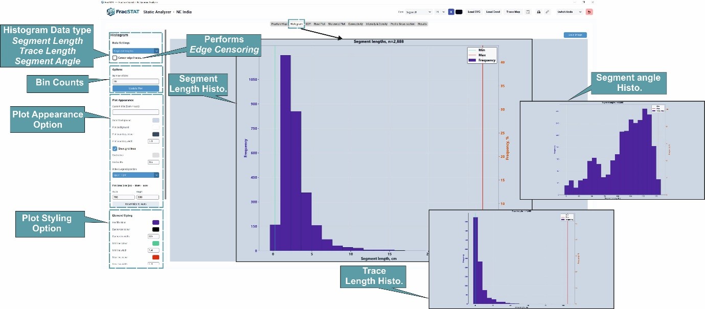
1.1 Sidebar Cards at a Glance
| Card | Purpose | Always visible? |
|---|---|---|
| Data Settings | Selects which quantity to plot (segment length, trace length, segment angle, or the bivariate Cross Plot) and whether edge‑censoring is applied. | Yes |
| Options | Sets the number of histogram bins and provides an explicit "Update Plot" redraw button. | Histogram modes |
| Plot Appearance | Controls the figure title, background colours, plot boundary styling, grid, legend placement, and the pixel dimensions of the plotting area. | Yes |
| Element Styling | Controls the histogram bar fill/border colours and the minimum/maximum reference‑line colours and widths. | Histogram modes |
| Text & Axis Styling | Controls the colour of the left (Frequency) axis text, the right (Frequency %) axis text, and the X‑axis text. | Histogram modes |
| Statistics | A read‑only results panel reporting n, censored count, minimum, maximum, mean, and total length. | Histogram modes |
| Cross Plot Settings | X‑axis/Y‑axis attribute selectors, colour‑by attribute, marker styling, trend‑line controls, and colour‑scale/colourbar options. | Cross Plot mode only |
1.2 Plot Canvas
The plot canvas is a Matplotlib Figure created with constrained_layout=True,
which automatically reserves space for axis labels, titles, and legends on every redraw rather than
relying on a single tight_layout() snapshot computed at build time. This matters
because the user can change the plot's pixel dimensions, its legend position, or add/remove the
right‑hand secondary axis (Frequency %) at any time, and the geometry needs to be recalculated
each time so labels are never clipped or overlapping.
In Histogram mode the canvas hosts two overlapping axes that share the same x‑axis: a primary (left) axis showing absolute frequency (bar counts) and a secondary (right, twinned) axis showing frequency as a percentage of the total sample. In Cross Plot mode the canvas hosts a single axis showing a scatter plot of two chosen attributes, with an optional colour‑mapped third attribute and an optional ordinary‑least‑squares trend line.
2. Data Input
2.1 Upstream Data Source
The Histogram Tab does not load files itself. It reads from two attributes maintained by the
parent StaticAnalyzerApp: self._static_results (preferred) and, as a
fallback, self.results. Both are pandas DataFrames populated by the Fracture Map
tab's geometry pipeline whenever an SVG trace map or an Excel/CSV orientation table is loaded and
the profile scale (width, length, and display unit) is applied.
Two broad data modalities are supported, distinguished internally by whether the loaded segments carry a pre‑set orientation rather than pixel geometry:
- SVG mode — each fracture trace is digitised as one or more straight segments with real pixel endpoints (X1, Y1, X2, Y2). Segment length and strike angle are derived directly from this geometry after pixel‑to‑real‑world scaling.
- Excel/CSV mode — fracture planes are supplied as tabular Strike/Dip (optionally with Length and Aperture columns) or as Trend/Plunge pole orientations converted to Strike/Dip. Because no true spatial geometry exists in this format, segment endpoints are synthetic (placed on a unit circle purely to preserve orientation for downstream calculations), and any Length/Aperture values come directly from optional spreadsheet columns rather than being derived from geometry.
2.2 Columns Consumed
| Column | Type | Used for | Notes |
|---|---|---|---|
Length_m | float | Segment‑length histogram; length statistics; Cross Plot "Segment Length" axis | Real‑world segment length in the currently selected display unit (despite the fixed column‑name suffix "_m"). Falls back to Length when Length_m is absent. |
StrikeDeg | float | Segment‑angle histogram; Cross Plot "Segment/Strike angle" axis | Stored fully‑directed (0–360°); the tab folds it to the 0–180° fracture‑orientation convention with modulo arithmetic before plotting. Falls back to SegmentAngle, then Angle, when StrikeDeg is absent. |
Trace | int | Trace‑length aggregation; edge‑censoring grouping | Used with a pandas groupby to sum segment lengths per trace. |
TraceLengthM | float | Trace‑length histogram (fast path) | Precomputed total length per trace when present; otherwise derived on demand via groupby("Trace")["Length_m"].sum(). |
X1, Y1, X2, Y2 | float | Edge‑censoring bounding‑box test; SVG fallback cross‑plot geometry | Real‑world (scaled) segment endpoints for SVG‑sourced data. |
Aperture | float | Cross Plot Y‑axis default for Excel/CSV data | Only populated when the source spreadsheet supplies an Aperture column; otherwise NaN. |
DipDeg | float | Cross Plot "Dip (°)" axis option | Falls back to a plain Dip column when DipDeg is absent. |
ID | int | Cross Plot "Segment ID" axis option | Sequential per‑segment identifier matching the Table/Results tabs. Falls back to a Segment column when ID is absent. |
2.3 Handling of Missing or Empty Data
If no data has been loaded (both self._static_results and self.results
are empty or None), both drawing routines display a centred, muted placeholder
message directly on the axes — "Load SVG or Excel data to plot distributions" or "Load data
first" — instead of raising an exception, and every entry in the Statistics card is reset to an
em‑dash. This defensive placeholder pattern is used throughout FracSTAT so that an empty project
never presents a blank or crashed plotting surface.
None values. Separately, in any Histogram mode, if enabling "Censor edge traces"
removes every remaining valid data point, the module shows "No valid data remaining after
censoring" rather than a blank or crashed histogram axis.
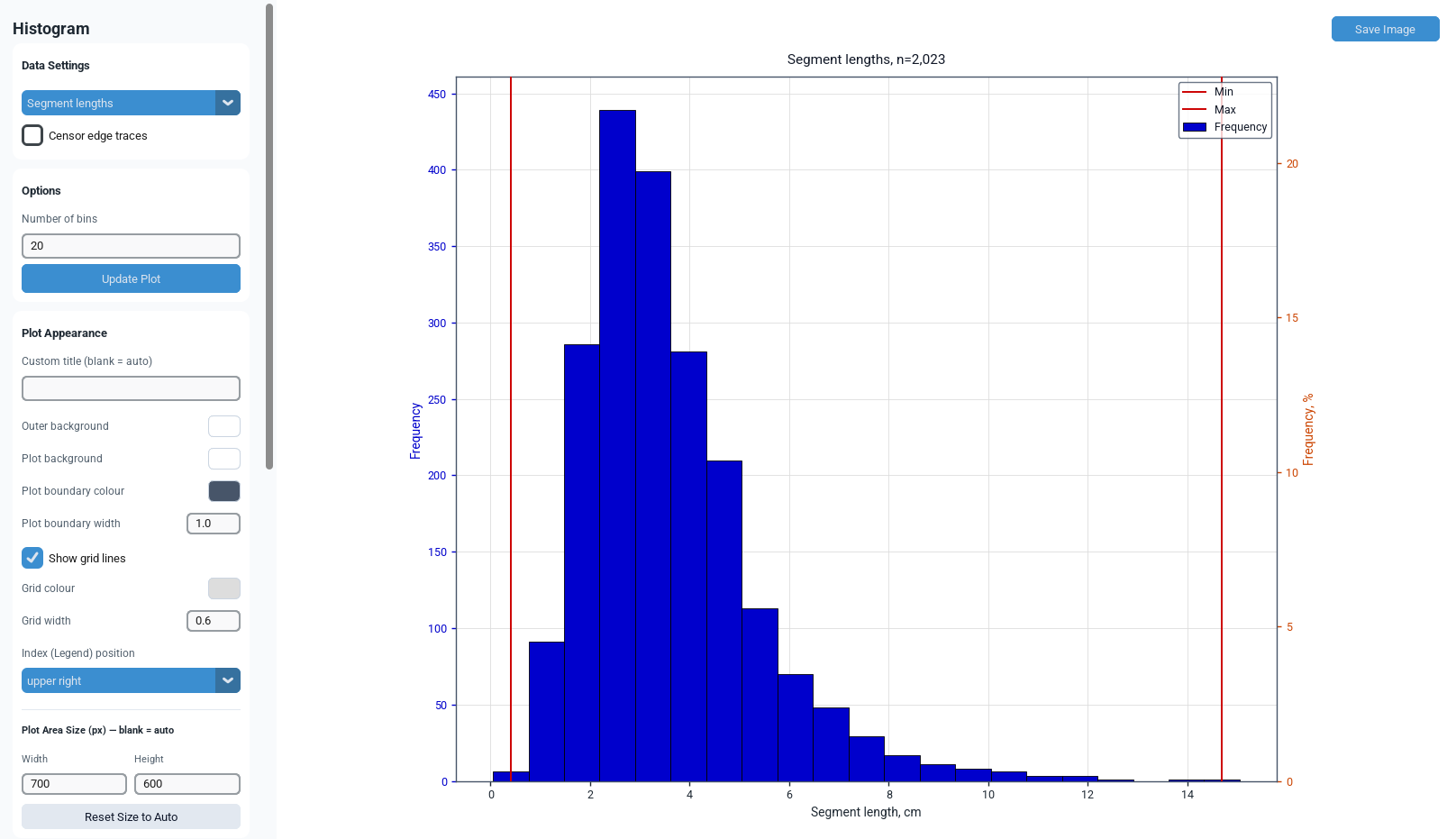
3. Settings and Controls, Card by Card
Unless stated otherwise, every control triggers an immediate redraw through the internal
dispatcher _dispatch_draw(), which routes to either the histogram renderer or the
cross‑plot renderer according to the current Data Settings selection.
3.1 Data Settings Card
| Control | Widget | Default | Effect |
|---|---|---|---|
| Data Settings dropdown | Option menu | Segment lengths | Chooses the plotted quantity: "Segment lengths", "Trace lengths", "Segment angles", or "Cross Plot". Selecting "Cross Plot" additionally reveals the Cross Plot Settings card; any other choice hides it. |
| Censor edge traces | Checkbox | Unchecked | When enabled, any trace with at least one segment endpoint numerically coincident with the bounding box of the loaded dataset is excluded from the plotted sample (see Section 5.2). Applies to Segment lengths, Trace lengths, and Cross Plot (SVG geometry only) modes. |
3.2 Options Card
| Control | Widget | Default | Valid range | Effect |
|---|---|---|---|---|
| Number of bins | Text entry | 20 | Clamped to 3–200 on commit | Sets the histogram bin count used to partition the length or angle range into equal‑width intervals. Committed on Enter or on focus‑out. |
| Update Plot | Button | — | — | Manually forces a redraw; provided for consistency of interaction pattern even though most controls already redraw automatically. |
3.3 Plot Appearance Card
| Control | Widget | Default | Effect |
|---|---|---|---|
| Custom title (blank = auto) | Text entry | "" (auto title) | Overrides the automatically generated plot title. The automatic title reports the plotted quantity and sample size n (and, in Cross Plot mode, the X/Y axis labels). |
| Outer background | Colour swatch | #FFFFFF | Sets the Matplotlib Figure facecolor — the canvas area outside the axes bounding box. |
| Plot background | Colour swatch | #FFFFFF | Sets the Axes facecolor (the area inside the plot frame). |
| Plot boundary colour | Colour swatch | #475569 | Sets the colour of all four Matplotlib spines (top, bottom, left, right). |
| Plot boundary width | Text entry (float) | 1.0 | Sets the line width of the plot spines, in points. |
| Show grid lines | Checkbox | Checked | Toggles the major gridlines on the primary axis. |
| Grid colour | Colour swatch | #DDDDDD | Sets the colour of the gridlines when shown. |
| Grid width | Text entry (float) | 0.6 | Sets the gridline width, in points. |
| Legend position | Option menu | upper right | One of: upper right, upper left, lower right, lower left, center, Outside Right, Outside Bottom, or None. "Outside Right"/"Outside Bottom" place the legend beyond the axes bounding box using a bbox_to_anchor offset; "None" suppresses the legend entirely. |
| Plot Area Size — Width (px) | Text entry (int) | 700 | Sets the target pixel width of the rendered figure by destroying and recreating the canvas at the requested size (see Section 5.4). |
| Plot Area Size — Height (px) | Text entry (int) | 600 | Sets the target pixel height of the rendered figure, using the same rebuild mechanism as Width. |
| Reset Size to Auto | Button | — | Rebuilds the canvas at the fixed default of 700 × 600 px (7.0 × 6.0 inches at 100 dpi). |
3.4 Element Styling Card (Histogram Modes)
| Control | Widget | Default | Applies to |
|---|---|---|---|
| Bar fill colour | Colour swatch | #0000CC | Histogram bars. |
| Bar border colour | Colour swatch | #000000 | The edge colour drawn around each bar. |
| Bar border width | Text entry (float) | 0.6 | Bar edge line width, in points. |
| Min line colour | Colour swatch | #CC0000 | The vertical reference line marking the sample minimum. |
| Min line width | Text entry (float) | 1.4 | Line width of the minimum‑value reference line. |
| Max line colour | Colour swatch | #CC0000 | The vertical reference line marking the sample maximum. |
| Max line width | Text entry (float) | 1.4 | Line width of the maximum‑value reference line. |
3.5 Text & Axis Styling Card (Histogram Modes)
| Control | Widget | Default |
|---|---|---|
| Frequency (Left) colour | Colour swatch | Matches Bar fill colour |
| Frequency % (Right) colour | Colour swatch | #CC4400 |
| X‑axis text colour | Colour swatch | Workspace text colour (typically #1F2933) |
3.6 Statistics Card
The Statistics card is a read‑only report, recomputed on every redraw from the filtered, positive‑valued sample. The displayed fields depend on the active plot mode.
Length Histogram Modes (Segment lengths / Trace lengths)
| Field | Description | Units |
|---|---|---|
| Max | Sample maximum of the plotted attribute. | display unit |
| Min | Sample minimum of the plotted attribute. | display unit |
| Median | Median value of the sample. | display unit |
| Mode | Most frequent value (dominant bin midpoint). | display unit |
| Std Dev | Standard deviation of the sample. | display unit |
Segment Angles Mode
| Field | Description | Units |
|---|---|---|
| Max | End of the shortest arc that contains every observed strike, traversed in the direction of increasing angle. This is the circular range endpoint, not max() — see Section 5.6. | degrees |
| Min | Start of that same shortest containing arc. Because the arc may wrap through 0°, Min can be numerically larger than Max; that is the correct reading of a wrapping quantity and not a fault. | degrees |
| CircMean | 180°‑periodic circular axial mean of strike angles, computed by double‑angle vector summation. | degrees |
| CircStdDev | Circular standard deviation of the strike distribution. | degrees |
| Dominant | Orientation of the modal bin (highest frequency). | degrees |
Min and Max in this mode are arc endpoints, not order statistics. The Min
and Max vertical reference lines on the plot mark the same two values, so on a set clustered
across 000° the pair of lines brackets the cluster instead of standing at the two edges of
the axis. The bin grid, by contrast, is still laid out over
min(θ)…max(θ) of the folded values, because that is a display span
over the plotted 0–180° domain rather than a statement about angular spread.
Cross Plot Mode
| Field | Description | Units |
|---|---|---|
| n (count) | Number of observations remaining in the plotted sample after filtering non‑finite and non‑positive values, and after any edge‑censoring. | count |
| Censored | Number of observations removed by the edge‑censoring rule (zero when censoring is disabled). | count |
| Minimum | Sample minimum of the plotted attribute. | display unit or degrees |
| Maximum | Sample maximum of the plotted attribute. | display unit or degrees |
| Mean | Arithmetic mean of the plotted attribute. | display unit or degrees |
| Total Length | Sum of all plotted lengths. | display unit |
3.7 Cross Plot Settings Card
This card is created hidden and is revealed only when the Data Settings dropdown is set to "Cross Plot"; toggling back to any histogram mode hides it again.
| Control | Widget | Default | Effect |
|---|---|---|---|
| X axis | Option menu | Segment Angle (°) | Selects the attribute plotted on the horizontal axis. Options: Segment Angle (°), Segment Length, Trace Angle (°), Trace Length, Strike (°), Length, Aperture (mm), Dip (°), Segment ID, Trace ID. |
| Y axis | Option menu | Segment Length | Selects the attribute plotted on the vertical axis, from the same option list as X axis. |
| Colour points by | Option menu | None | Optionally colours each scatter point by a third attribute using a continuous colormap; "None" plots all points in a single solid colour. Options: None, Segment Angle (°), Segment Length, Trace Angle (°), Trace Length, Strike (°), Length, Aperture (mm), Dip (°), Trace ID. |
| Custom title (blank = auto) | Text entry | "" | Overrides the automatic "X‑label vs Y‑label (n=...)" title. |
| Dot colour | Colour swatch | #2563EB | Marker colour used when "Colour points by" is "None". |
| Dot size | Text entry (float) | 18 | Marker area, in points², passed to Matplotlib's scatter s parameter. |
| Dot opacity (0–1) | Text entry (float) | 0.7 | Marker alpha, clamped to [0, 1]. |
| Show trend line (OLS) | Checkbox | Unchecked | Fits and overlays an ordinary‑least‑squares regression line through the plotted points (requires ≥ 2 points); see Section 4.3. |
| Trend line colour | Colour swatch | #DC2626 | Colour of the OLS regression line. |
| Trend line width | Text entry (float) | 1.8 | Line width of the OLS regression line, in points. |
| Colour scale (when colouring by) | Option menu | viridis | Matplotlib colormap name applied when "Colour points by" is not "None". Options include viridis, plasma, inferno, magma, cividis, turbo, jet, hot, coolwarm, RdYlBu, Spectral, YlGnBu, Greys. |
| Colorbar position | Option menu | Right | Right, Left, Bottom, Top, or None; controls placement of the colourbar associated with the "Colour points by" mapping. |
| Colorbar bg colour | Colour swatch | Matches Outer background | Background colour behind the colourbar axis. |
_label_with_unit helper. Every other
option (angles, Aperture, Dip, IDs) is shown with its label unchanged, since those attributes
are not affected by the display‑unit setting.
4. Mathematical Background
4.1 Segment Length and Segment Angle Derivation
For SVG‑sourced segments, each fracture segment i has real‑world endpoint coordinates (x1, y1) and (x2, y2) after pixel‑to‑unit scaling. Two scalar attributes are used throughout the Histogram Tab:
The negation of the y‑component accounts for the fact that SVG/screen coordinate systems increase downward, whereas the geological azimuth convention (0° = up‑page / north‑referenced) increases in the opposite sense. The resulting angle is reduced modulo 180° because fracture strike is an axial (undirected line) quantity — a segment trending 040° is geometrically identical to one trending 220°.
This raw‑geometry fallback also respects the same workspace structural‑map adjustments that
the Fracture Map tab's own geometry pipeline applies, so an angle recomputed here from
endpoints always agrees with the pre‑computed StrikeDeg value for the same
segment regardless of how the map has been reoriented:
The Flip X and Reverse Y toggles and the
Y‑axis azimuth‑from‑North value are read live from the Fracture Map tab's own
settings (_static_map_flip_x_var, reverse_y_var, and
_static_map_y_axis_north_var respectively); if any of these are unavailable the
module falls back to no flip, Y reversed, and 0° azimuth. Without this adjustment, a
Segment Angle computed from raw coordinates would silently ignore the workspace's Flip X,
Flip Y, and north‑referencing settings and disagree with every other angle shown elsewhere in
the application whenever those settings differed from their defaults.
StrikeDeg column already exists in
the results table (the normal case, since this angle is computed once by the Fracture Map tab's
geometry pipeline and reused by every downstream tab), the Cross Plot "Segment Angle (°)" option
simply reads and folds that column rather than recomputing it from raw coordinates; the
raw‑geometry computation above is used only as a fallback for legacy or partially restored
sessions in which the endpoint columns exist but the derived StrikeDeg column does
not.
4.2 Histogram Binning
Given the filtered, positive sample {L₁, ..., Lₙ} and a user‑selected bin count nBins, the module constructs equal‑width bins centred on a grid that starts at the sample minimum and ends at the sample maximum:
The requested bin count is a step count, not a bar count. Because the centre grid includes both endpoints, nBins produces nBins + 1 bars, and the plotted span overhangs the data by half a step at each end. Entering 20 bins therefore yields 21 bars. This matters when reproducing a figure in another package or comparing bar heights against an externally computed histogram of the same data.
Bin counts Ck are then obtained with a standard histogram accumulation (numpy.histogram)
over these edges (Harris et al., 2020).
In the degenerate case Lmin = Lmax (every observation identical, or n = 1), the
module falls back to a single bin of unit width centred on that value, avoiding a division by
zero in the step calculation.
The bin count is a free parameter, and no automatic rule is applied. The value entered is used as given; FracSTAT does not compute a data-driven bin width such as Sturges' rule (Sturges, 1926), Scott's rule (Scott, 1979), or the Freedman–Diaconis rule (Freedman and Diaconis, 1981), each of which selects a width that balances resolution against sampling noise. Because fracture-length samples are usually strongly right-skewed, the classical rules — derived under near-normal assumptions — tend to be conservative for this kind of data, and inspecting two or three bin counts before choosing one is more reliable than trusting any single value.
In Segment angles mode the bin grid and the reported extremes come from different
quantities. Lmin and Lmax above are the plain min()/max()
of the folded angles and continue to set the bin grid, because that is a display span over
the plotted 0–180° domain. The Min and Max values on the Statistics card and the two
reference lines instead come from the circular range (Section 5.6). The two
are intentionally different: one is where to draw the axis, the other is what the angular
spread actually is.
Two vertical axes are always displayed together: the left axis shows the raw count Ck, and the right (twin) axis shows the same information rescaled to percentage of the total sample:
The 1.05 multiplier provides a 5% headroom margin above the tallest bar so that the bar outline is never clipped against the top of the plotting frame. Because both axes are tied to the same underlying bar heights, they are always mutually consistent — the percentage axis is a pure linear rescaling of the count axis, not an independently binned distribution.
n = lengths.size
nBins = self._length_bins()
lmin, lmax = lengths.min(), lengths.max()

if mode == "Segment angles":
    # Reported/marked extremes come from the circular range, because
    # min() and max() of a mod-180 quantity describe the coordinate cut
    # rather than the fractures.  lmin/lmax still set the bin grid,
    # which is a display span over the plotted 0-180 domain.
    extreme_min, extreme_max = self._axial_arc_extremes(lengths)
else:
    extreme_min, extreme_max = float(lmin), float(lmax)

if lmin == lmax:
    bin_edges = [lmin - 0.5, lmax + 0.5]
    counts, centres, widths = [len(lengths)], [lmin], [1.0]
else:
    step = (lmax - lmin) / nBins
    centres = np.arange(lmin, lmax + step/2, step)
    bin_edges = np.concatenate([[centres[0] - step/2], centres + step/2])
    counts, _ = np.histogram(lengths, bins=bin_edges)
    widths = np.diff(bin_edges)

ax_left.bar(centres, counts, width=widths, align="center",
            color=hist_col, edgecolor=b_edge_col, linewidth=b_edge_lw,
            label="Frequency")

ax_right = ax_left.twinx()
count_max = counts.max() if counts.max() > 0 else 1
ax_right.set_ylim(0, count_max / n * 100.0 * 1.05)
Simplified excerpt of the binning and dual‑axis logic in _draw_length_histogram(), showing the degenerate single‑bin fallback and the percentage‑axis headroom calculation described above.
4.3 Cross‑Plot Ordinary Least‑Squares Trend Line
When "Show trend line (OLS)" is enabled, the module fits a first‑degree polynomial (a straight
line) to the plotted (x, y) pairs using numpy.polyfit, which solves the ordinary
least‑squares normal equations for slope m and intercept b:
The fitted line is drawn across the full observed x‑range [min(x), max(x)] and its legend entry reports the equation and R² to three decimal places: "OLS y = m·x + b, R² = value". Because the OLS fit and the R² statistic both assume a linear relationship and are sensitive to outliers and heteroscedasticity, they should be interpreted as a descriptive summary of linear association rather than a formal hypothesis test unless the regression assumptions (residual normality, homoscedasticity, absence of leverage points) have been independently verified.
A linear fit is the wrong model for most fracture scaling relationships. Aperture–length, displacement–length, and comparable relationships in rock are generally reported as power laws of the form a ∝ Ln, with the exponent itself the quantity of interest and estimates of n ranging from sublinear to approximately linear depending on the mechanism and dataset (Vermilye and Scholz, 1995; Olson, 2003; Schultz et al., 2008). Fitting a straight line on linear axes estimates none of these exponents. Where a scaling exponent is the objective, the appropriate procedure is a regression in log–log space with explicit treatment of truncation and censoring (Pickering et al., 1995); neither the log transform nor those corrections is applied by this tab.
4.4 Angle Wrapping and Axial Statistics
All angular quantities handled by the Histogram Tab (StrikeDeg, Strike (°), Trace Angle (°),
Segment Angle (°)) are folded to the axial 0–180° domain via the modulo operator
(value % 180.0) at the point of column resolution, consistent with the
fracture‑orientation convention used throughout the Static Analyzer. When the plot mode is set
to Segment angles, the tab computes and displays the circular axial mean
(CircMean) and circular standard deviation (CircStdDev) using 180°‑periodic double‑angle vector
summation (Mardia and Jupp, 2000, §2.3.2),
together with the dominant bin orientation (Dominant), directly on the Statistics
card. For length‑weighted axial mean strike, consult the Rose Plot tab, which implements the
same circular‑statistics formula weighted by segment length.
The dispersion measure is the circular standard deviation derived from the mean resultant length R̄, halved to return it to the axial domain:
This is the standard circular standard deviation of Mardia and Jupp (2000, §2.3.4) and Fisher (1993, §2.3.1). It is unbounded as R̄ → 0: a perfectly uniform set of orientations drives R̄ toward zero and s toward very large values, which is the correct behaviour for the formula but means a large CircStdDev should be read as "no preferred orientation" rather than as a literal angular spread. The implementation floors R̄ at 10⁻¹² to keep the logarithm finite.
Wrapping also invalidates the ordinary extremes. On a mod‑180° coordinate, min()
and max() are decided by where the coordinate happens to have been cut, not by the
data: a population clustered on 000° has members just under 180° and just over 0°, so the
arithmetic pair reports "Min 0.1°, Max 179.9°" — an apparent spread of the entire domain — for
fractures whose real angular spread may be two degrees. The well‑defined replacement is the
circular range, the shortest arc containing every observation:
following Fisher (1993, §2.3.3) and Mardia and Jupp (2000, §2.3.2). The returned pair traverses the arc in the direction of increasing angle and may wrap through the origin, exactly as the orientations do; the algorithm is given in Section 5.6. Note that neither the plain extremes nor the circular range is a robust statistic — a single stray outlier still controls the arc — so the circular range describes the sample's angular support, not the concentration of the population, for which CircStdDev is the appropriate measure.
5. Algorithms
5.1 Data‑Source Selection and Attribute Resolution
The private helper _cross_col(df, axis_label) is the central attribute‑resolution
routine used by Cross Plot mode. Given a human‑readable axis label (e.g. "Segment Length",
"Strike (°)"), it performs the following steps:
- Normalise the label by stripping any parenthetical unit suffix (e.g. "(°)") and collapsing whitespace, then case‑fold it for comparison.
- Attempt to resolve the corresponding DataFrame column directly (e.g. StrikeDeg, Length_m, Aperture, DipDeg, ID, Trace), tolerating either the modern FracSTAT export naming or common synonyms.
- For "Segment Angle" and "Segment Length" specifically, fall back to reconstructing the value from raw SVG endpoint columns (X1, Y1, X2, Y2) if the derived column is absent — this occurs for older or partially restored project sessions that predate a schema change.
- For "Trace Angle" and "Trace Length", aggregate per‑trace values using a pandas
groupbyon the Trace column (mean strike per trace, or summed length per trace) rather than reading a per‑segment value directly. - Return
Noneif no resolution path succeeds, allowing the caller to attempt a further SVG‑geometry fallback or, failing that, present the "axis not available" empty state.
5.2 Edge‑Censoring Algorithm
Real fracture‑trace datasets digitised from a finite map or photograph are subject to a well‑known sampling bias: traces truncated by the edge of the mapped area have an artificially shortened observed length compared to their true (unknown) extent. The "Censor edge traces" option implements a geometric detection of this condition:
- Compute the bounding box of the entire loaded dataset: xmin, xmax from the union of X1/X2, and ymin, ymax from the union of Y1/Y2.
- Define a tolerance proportional to the extent of each axis:
tol_x = max((xmax − xmin) × 10⁻⁶, 10⁻⁶)and likewise for tol_y. This scales the numerical comparison to the physical size of the map rather than using a fixed absolute tolerance, which would be either too strict (missing genuine boundary touches after floating‑point rounding) or too permissive (falsely censoring interior traces). - For every segment, test whether any of its four coordinate values (X1, X2, Y1, Y2) lies within tolerance of the corresponding bounding‑box extreme, using
numpy.isclosewith the computed absolute tolerance. - Identify the set of distinct Trace identifiers that contain at least one such boundary‑touching segment.
- Remove every segment belonging to any flagged trace from the plotted sample (not just the touching segment), and report the number of removed segments (Histogram modes) or removed traces (Trace‑length mode) as the "Censored" statistic.
5.3 SVG Geometry Reconstruction for Cross Plots
The helper _svg_cross_dataframe() rebuilds a minimal geometry table directly from
the in‑memory Segment objects (bypassing the asynchronous results table) whenever that table is
unavailable or incomplete for the requested axis pair. Because raw SVG segment coordinates are
expressed in arbitrary drawing‑tool pixel units, this routine re‑applies the same
pixel‑to‑real‑world scaling used by the main geometry pipeline:
profile_width and profile_length are read from the Fracture Map tab's
own sidebar fields (defaulting to 260 and 100 respectively if those widgets are not yet
initialised). This ensures that a Cross Plot "Segment Length" computed via this fallback path is
expressed in the same physical scale as the Length_m column used elsewhere in the
application, rather than in unscaled pixel units.
5.4 Canvas Rebuild Algorithm (Custom Plot Sizing)
Because the embedded FigureCanvasTkAgg does not support changing a live canvas's
backing pixel dimensions in place without artefacts, the "Plot Area Size" controls operate
through a full tear‑down‑and‑rebuild sequence, implemented in
_len_rebuild_canvas(w_in, h_in, dpi):
- Destroy the existing Qt canvas widget.
- Close the existing Matplotlib Figure object via
matplotlib.pyplot.close()to release its internal renderer resources and avoid a slow memory leak across repeated resizes. - Construct a new Figure at the requested size in inches (converted from the requested pixel dimensions at the fixed 100 dpi used throughout FracSTAT) with
constrained_layout=True, and a new single Axes. - Construct a new
FigureCanvasTkAggbound to the new Figure, re‑attach the button‑release event handler used for legend‑position persistence, and grid it into the existing plot card. - Invoke the drawing dispatcher to repopulate the new canvas with the current data and settings.
The width and height entry fields also drive an aspect‑ratio lock
(ax.set_box_aspect(h_px / w_px)) applied after each redraw, which keeps the plotted
box's aspect ratio consistent with the requested pixel dimensions even though constrained_layout
is otherwise free to adjust axis position.
5.5 Draggable Legend / Trend‑Line Legend Position Persistence
When FracSTAT's global "Move Elements" editing mode is active, the Matplotlib legend on the
histogram or cross‑plot axes becomes draggable. To ensure a manually dragged legend does not
snap back to its default corner on the next redraw, the module records the legend's
bounding‑box position — in axes‑fraction coordinates — on every mouse‑button‑release event, and
reuses that stored anchor point (bbox_to_anchor with loc='lower left')
on all subsequent redraws until the legend position preset in the Plot Appearance card is
explicitly changed, at which point the stored anchor is cleared and the newly selected preset
position takes over.
5.6 Circular Range of Axial Angles (_axial_arc_extremes)
The static helper _axial_arc_extremes(angles_deg, period=180.0) returns the
endpoints of the shortest arc containing every axial angle, and supplies the Min and Max values
of Segment angles mode (Section 3.6) and the two vertical reference lines.
- Fold to the period and sort: discard non‑finite values, reduce the rest modulo 180°, sort ascending.
- Return
(0.0, 0.0)for an empty sample and(θ, θ)for a single observation. - Compute the gaps between successive sorted angles, and separately the wrap gap
(θ₁ + 180°) − θ_nthat spans the cut at the origin. - Find the widest of the successive gaps.
- If the wrap gap is at least as wide as that widest interior gap, the sample already occupies one unbroken run inside the domain and the plain extremes are the arc endpoints — return
(θ₁, θ_n). - Otherwise the widest empty sector lies inside the domain, so the containing arc is its complement and wraps through the origin — return
(θ_{k+1}, θ_k), the angle immediately after the gap as the start and the angle immediately before it as the end.
angles = np.sort(angles[np.isfinite(angles)] % period)
if angles.size == 0:
    return 0.0, 0.0
if angles.size == 1:
    return float(angles[0]), float(angles[0])

gaps     = np.diff(angles)
wrap_gap = (angles[0] + period) - angles[-1]
widest   = int(np.argmax(gaps))

if wrap_gap >= gaps[widest]:
    # The widest empty sector already straddles the cut, so the sample
    # occupies one unbroken run and the plain extremes are correct.
    return float(angles[0]), float(angles[-1])
return float(angles[widest + 1]), float(angles[widest])
The tie condition wrap_gap >= gaps[widest] uses >= deliberately: when
the two candidate sectors are equally wide the arc is ambiguous, and preferring the non‑wrapping
answer keeps the reported pair in ascending order for the common case of a sample that does not
actually straddle the cut. The step is applied only in Segment angles mode; length modes take
float(min) and float(max) unchanged, since length does not wrap.
6. Statistical Methods
| Statistic | Formula | Interpretation |
|---|---|---|
| n | count of filtered, positive observations | Effective sample size available for interpretation; small n (roughly below 30) warrants caution when generalising the distribution shape. |
| Minimum / Maximum (lengths) | min(x), max(x) | Bounds of the observed range; in fracture studies the minimum is frequently a mapping‑resolution artefact (the shortest resolvable trace) rather than a true geological minimum. |
| Min / Max (angles) | endpoints of the shortest containing arc (Section 5.6) | Angular support of the sample, wrap‑aware. Not order statistics: the pair may run "backwards" (Min > Max) when the arc crosses 0°, and the difference Max − Min must be taken modulo 180° to recover the circular range. |
| Mean | (1/n) Σ xi | Central tendency; for heavy‑tailed (power‑law‑like) fracture length distributions the mean can be strongly influenced by a small number of very long traces and may not represent a "typical" fracture — the CDF tab's median and quantile statistics are often more robust. |
| Total Length / Sum | Σ xi | Aggregate fracture length in the sample area; directly relevant to fracture‑intensity metrics such as P21 computed elsewhere in FracSTAT (Intensity & Density tab). |
| Censored count | count of excluded boundary‑touching observations | Quantifies the magnitude of the truncation‑bias correction; a large censored fraction relative to n signals that the mapped area may be too small relative to the characteristic fracture length for unbiased length statistics (Priest and Hudson, 1981). |
These are sample statistics, reported without uncertainty. No standard errors, confidence intervals, or goodness-of-fit measures accompany them, and no test is performed against any distributional model. Interval estimates for the mean of a heavy-tailed sample generally require a resampling approach rather than a normal approximation (Efron and Tibshirani, 1993); the CDF tab, not this one, provides that machinery (Section 6.1).
6.1 Relationship to the CDF Tab
The Histogram Tab intentionally limits itself to elementary descriptive statistics and
equal‑width binning. Rigorous distributional inference — maximum‑likelihood fitting of power‑law,
exponential, log‑normal, Weibull, or truncated power‑law models; Kolmogorov–Smirnov
goodness‑of‑fit; information‑criterion model selection; and bootstrap confidence intervals — is
the responsibility of the dedicated CDF tab, which operates on the same underlying
Length_m / TraceLengthM data. Analysts requiring a defensible power‑law
exponent or a formal comparison between candidate distributional models should proceed to the
CDF tab rather than inferring such conclusions from the equal‑width histogram alone, since bin
width and placement are well known to bias the visual appearance of heavy‑tailed distributions
(Clauset et al., 2009). Estimating a
power-law exponent by regressing on binned frequencies — the procedure a histogram invites — is
known to be biased, and maximum-likelihood estimation on the unbinned data is the recommended
alternative (Clauset et al., 2009).
6.2 Cross‑Plot Regression Diagnostics
The R² value reported alongside the OLS trend line is the squared Pearson product‑moment
correlation coefficient between the plotted x and y arrays, computed via
numpy.corrcoef. It quantifies only the proportion of variance in y that is linearly
associated with x for the specific pair of attributes currently selected; it does not by itself
establish causation, and a low R² does not preclude a genuine non‑linear or threshold
relationship (many aperture–length relationships in the fracture‑mechanics literature follow
power‑law rather than linear scaling
(Vermilye and Scholz, 1995;
Olson, 2003), in which case a log–log
transformation prior to interpretation — not currently automated by this tab — would be more
appropriate).
7. Visualization & Figure Components
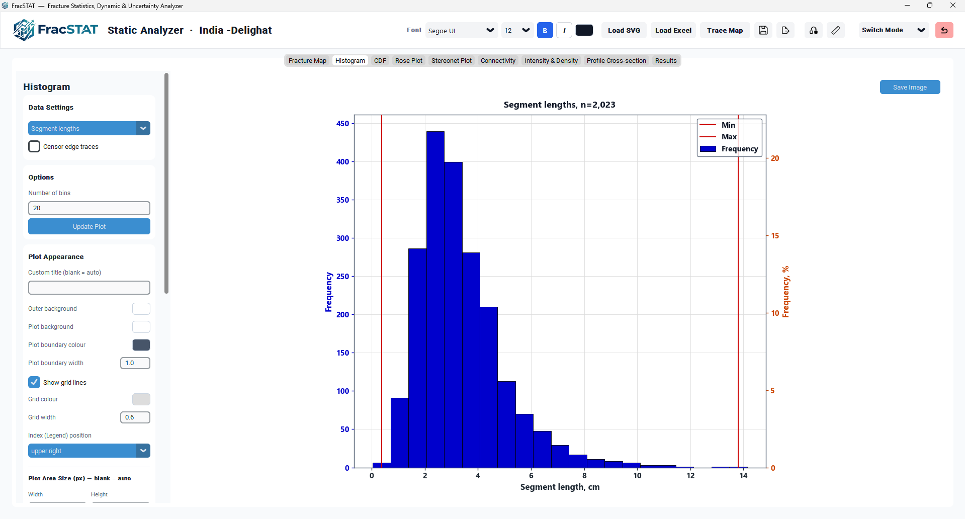
7.1 Histogram Figure Components
- Bars — one bar per bin, centred on the bin midpoint, width equal to the bin step, coloured and outlined per the Element Styling card.
- Left y‑axis (Frequency) — absolute bin counts, labelled and coloured per the Text & Axis Styling card, with an integer‑only tick locator so fractional count ticks never appear.
- Right y‑axis (Frequency, %) — the same bar heights rescaled to percentage of n, sharing the x‑axis via a twin axis.
- Minimum/Maximum reference lines — full‑height vertical lines marking the sample extremes, each with its own colour and width and included in the legend. In Segment angles mode they mark the endpoints of the shortest containing arc instead (Section 5.6), so they can appear inside the cluster rather than at the edges of the axis.
- Title — automatically composed from the selected mode and sample size, e.g. "Segment lengths, n=1,204", with censored‑count annotation appended when applicable; replaced verbatim by the Custom Title field when non‑blank.
- Z‑order correction — because Matplotlib's twin axis by default stacks the new (right) axis above the original, the tab explicitly reassigns z‑order and patch visibility so the left axis (and therefore its legend) remains clickable and visible in front of the right‑axis background.
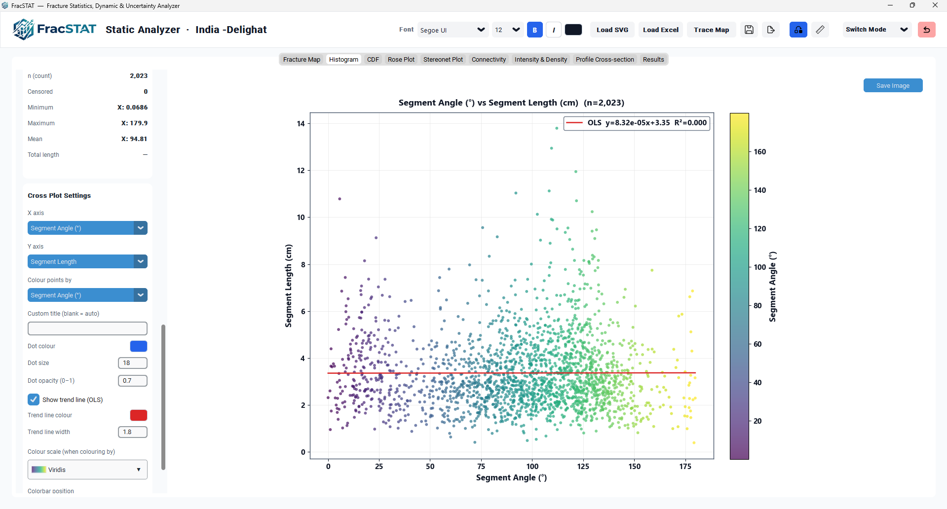
7.2 Cross‑Plot Figure Components
- Scatter markers — either solid‑coloured or continuously colour‑mapped by the selected third attribute.
- Colourbar — rendered on the requested side (Right/Left/Bottom/Top) only when a colour‑by attribute is active, labelled with that attribute's name.
- OLS trend line (optional) — a single straight line spanning the observed x‑range, with a legend entry reporting the fitted slope, intercept, and R².
- Title, axis labels, spines, and gridlines — styled identically in spirit to the histogram mode, using the same Plot Appearance controls.
7.3 Save Image
The "Save Image" toolbar button calls the shared save_plot_image() helper
(implemented once in the parent StaticAnalyzerApp and reused by every tab), which
writes the current Figure to a timestamped PNG file inside a per‑project
"FracSTAT_plot_exports" folder at the export DPI configured in the application Settings page
(default 300 dpi), using bbox_inches='tight' so that any externally positioned
legend or annotation is not clipped from the saved image.
8. Step‑by‑Step Example Workflows
8.1 Example 1 — Segment‑Length Distribution from an SVG Trace Map
- In the Fracture Map tab, load an SVG containing digitised fracture traces and confirm the profile width/length and display unit are correctly calibrated.
- Switch to the Histogram Tab. The Data Settings dropdown defaults to "Segment lengths".
- Set "Number of bins" to a value appropriate to the sample size — a common heuristic is nBins ≈ √n or nBins ≈ 1 + log₂(n) (Sturges' rule), though the module does not enforce either automatically and leaves the choice to the analyst.
- Enable "Censor edge traces" if the mapped area is known to be smaller than the characteristic fracture length, to reduce truncation bias in the reported Mean and Total Length statistics.
- Record the Statistics card's n, Minimum, Maximum, Mean, and Total Length values for the project report, and use "Save Image" to export a publication‑ready PNG of the histogram.
8.2 Example 2 — Comparing Segment vs Trace Length
Switching the Data Settings dropdown between "Segment lengths" and "Trace lengths" on the same loaded dataset allows a direct comparison between the length distribution of individual digitised segments (influenced by how finely a curved trace was sampled during digitisation) and the length distribution of complete traces (summed across all of a trace's constituent segments). A pronounced discrepancy between the two — for example, a segment‑length histogram dominated by very short bins while the trace‑length histogram shows a broader spread — can indicate over‑segmentation of curved traces during the SVG tracing step (see the Trace Map tool's "Curve step" parameter) rather than a genuine geological signal.
8.3 Example 3 — Cross‑Plotting Length against Aperture
- Load an Excel/CSV fracture‑plane table containing Length (m) and Aperture (mm) columns.
- In the Histogram Tab, set Data Settings to "Cross Plot".
- Set X axis to "Segment Length" and Y axis to "Aperture (mm)" (these are the pre‑selected defaults whenever Excel/CSV data with these columns is detected).
- Enable "Show trend line (OLS)" to obtain a first‑order linear length–aperture scaling estimate and its R² for the loaded population; note the caveat in Section 6.2 regarding non‑linear (e.g. power‑law) length–aperture scaling relationships commonly reported in the fracture‑mechanics literature.
- Optionally set "Colour points by" to "Strike (°)" to visually assess whether length–aperture scaling differs systematically between orientation sets.
9. Geological Interpretation
9.1 Fracture Length Distributions
Fracture (and joint, vein, and fault) length populations in nature are widely documented to follow heavy‑tailed distributions — commonly approximated by power‑law, log‑normal, or truncated power‑law forms over some intermediate range of scales — reflecting scale‑invariant growth and coalescence processes during fracture propagation (Bonnet et al., 2001). A histogram that appears strongly right‑skewed, with most bars concentrated at short lengths and a long thin tail of rare, very long traces, is consistent with this expectation and should motivate a follow‑up analysis in the CDF tab rather than being taken as evidence of a log‑normal or exponential process from visual inspection alone, since equal‑width linear binning tends to obscure power‑law tail behaviour that is only clearly visible on logarithmic axes (Clauset et al., 2009). Note also that power-law scaling in real fracture populations holds only over a finite range of scales, and is bounded below by mapping resolution and above by the size of the sampled area (Bonnet et al., 2001; Marrett et al., 1999).
9.2 Truncation and Censoring Bias
Because any finite outcrop, borehole image, or remotely sensed map necessarily has edges, fractures that would naturally extend beyond the mapped area are recorded with an artificially shortened apparent length. The distinction is conventionally drawn between censoring, the underestimation of traces cut off at a boundary, and truncation, the under-representation of short traces below the resolution limit; both distort length statistics and both bias a power-law exponent estimated without correction (Pickering et al., 1995; Priest and Hudson, 1981). The edge‑censoring feature provides a first‑order correction for the former by removing affected traces entirely from the length statistics, trading a reduction in sample size for an improvement in the accuracy of the remaining Mean and Total Length values. Analysts working with small mapped areas relative to the expected fracture length scale should treat the uncensored Mean length statistic with particular caution, since it will systematically underestimate the true population mean.
Discarding censored traces is not an unbiased estimator. Removing every boundary-touching trace also removes the longest members of the population preferentially, because long traces are more likely to reach a boundary. The remaining sample is cleaner but still biased low, and the bias grows as the mapped area shrinks relative to the characteristic fracture length. Formal treatments that estimate the underlying length distribution from censored window observations, rather than discarding them, are given by Mauldon (1998) and Zhang and Einstein (2000); those estimators are not implemented here.
9.3 Segment Angle Histograms and Structural Sets
The Segment angles histogram mode provides a linear‑axis (as opposed to the Rose Plot tab's polar/equal‑area) view of the strike‑angle distribution, folded to the 0–180° axial convention. Multiple distinct peaks (modes) in this histogram are typically diagnostic of multiple structural fracture sets formed under different regional or local stress orientations, or of a single set overprinted by a later, differently oriented set (Peacock et al., 2016). The reported summary statistics are wrap‑aware: CircMean and CircStdDev use 180°‑periodic double‑angle summation, and Min/Max are the endpoints of the shortest containing arc (Section 4.4). The bars, however, are not — the bin grid is a linear partition of the folded 0–180° domain, so a population whose true dominant orientation straddles the 0°/180° boundary is split between the first and last bins and can appear artificially bimodal in this view even though CircMean correctly reports a single mode. Where the histogram and CircMean disagree in that way, the wrap is the explanation and CircMean is the statistic to trust; the Rose Plot tab's polar representation shows the same population without the artificial split, and is the more reliable view for near‑boundary orientation sets.
9.4 Length–Aperture and Length–Attribute Cross Plots
Positive correlations between fracture length and aperture are frequently reported in the structural geology and reservoir engineering literature and are commonly interpreted in terms of linear elastic fracture mechanics scaling relationships between fracture length and displacement/aperture (Vermilye and Scholz, 1995; Scholz, 2010), although reported exponents vary and sublinear scaling is common (Olson, 2003). The relationship matters beyond descriptive interest: because flow through a fracture scales roughly with the cube of aperture, an aperture–length correlation propagates strongly into network-scale permeability (Klimczak et al., 2010). The Cross Plot tool's OLS trend line and R² provide a rapid first assessment of such a relationship within a given dataset, but formal scaling‑law exponent estimation (which requires a log–log regression and awareness of the truncation and censoring effects discussed in Section 9.2) should be pursued using dedicated statistical tools outside FracSTAT if publication‑quality scaling exponents are required.
10. Limitations
| Limitation | Description |
|---|---|
| Edge‑censoring is a simple heuristic | It is a boundary‑proximity test based on the dataset's own bounding box; it cannot detect truncation against an irregular (non‑rectangular) mapped‑area boundary, nor truncation caused by cloud cover, image saturation, or other non‑geometric data‑quality limitations. |
| Censoring is handled by exclusion, not estimation | Boundary-touching traces are discarded rather than used to estimate the underlying length distribution, which preferentially removes long traces and leaves a residual low bias (Section 9.2). Window-based estimators that retain censored observations are described by Mauldon (1998) and Zhang and Einstein (2000). |
| No correction for resolution truncation | Short traces below the mapping or digitisation resolution are simply absent from the sample. No lower truncation limit is estimated or reported, so the shape of the small-length end of the histogram reflects the mapping process as much as the geology (Pickering et al., 1995). |
| Binning is linear, not circular | Segment‑angle summary statistics are wrap‑aware (circular axial mean and standard deviation, and a circular‑range Min/Max), but the histogram bins themselves are a linear partition of the folded 0–180° domain. A set straddling 0°/180° is therefore split across the two end bins and may read as bimodal; cross‑check against CircMean and the Rose Plot tab. |
| Circular range is not robust | The shortest containing arc is fixed by the two observations bounding the widest empty sector, so one stray strike widens it as much as a genuinely dispersed population would. It measures angular support, not concentration — use CircStdDev for the latter. |
| Angle bin grid spans the observed values, not the full domain | Bin edges run from min(θ) to max(θ) of the folded sample rather than a fixed 0–180° axis, so the horizontal extent of the bars differs between datasets and the bar positions of two histograms are not directly comparable without setting axis bounds manually. |
| No automatic bin-width rule | The bin count is taken as entered. Standard data-driven rules (Sturges, 1926; Scott, 1979; Freedman and Diaconis, 1981) are not offered, so the visual impression of the distribution remains partly under user control. |
| No uncertainty on any statistic | Means, sums, and circular statistics are point estimates without standard errors or confidence intervals, and no test against a distributional model is performed. Interval estimates for heavy-tailed samples require resampling (Efron and Tibshirani, 1993); see the CDF tab. |
| Cross-plot fit is linear only | The trend line is an OLS fit on linear axes with a Pearson R². It cannot estimate a power-law scaling exponent, which is the form these relationships usually take (Olson, 2003). |
11. Advanced & Related Capabilities
11.1 Legacy Column and Unit Compatibility
The attribute‑resolution logic explicitly strips a stray "Â" character sequence and collapses whitespace before matching labels, guarding against the case where the degree symbol (°) has been mis‑decoded through a legacy Windows text encoding path. It also recognises both singular and pluralised historical label variants (e.g. "Trace Angle" vs "Trace Angles"), so previously saved project sessions or exported CSVs that used an older label convention continue to resolve correctly.
11.2 Automatic Default Correction for Mixed Sessions
Because the two supported data modalities (SVG vs Excel/CSV) have different natural default Cross Plot axis pairs, the module detects and silently corrects the situation where a Cross Plot was opened before an SVG file had finished loading — in which case the widgets could still hold the Excel‑oriented default pair, Segment Length vs Aperture (mm), which has no meaning for SVG‑only data — and resets them to the SVG‑appropriate default pair, Segment Angle (°) vs Segment Length, immediately before resolving columns for that redraw.
11.3 Performance Notes
- Constrained layout over manual
tight_layout()— recomputes label/legend spacing analytically on every draw, which is more robust than a single post‑hoc pass when the user is actively changing dimensions, legend position, or the secondary percentage axis. - Deferred redraw via
draw_idle()— schedules a repaint on the UI event loop rather than forcing an immediate synchronous render, letting several rapid successive setting changes coalesce into fewer actual repaints. - On‑demand Cross‑Plot geometry reconstruction — the SVG‑geometry fallback path is only invoked when the primary results table is unavailable, incomplete, or the requested axis pair is the special‑cased Segment‑Angle/Segment‑Length combination for SVG data, avoiding redundant per‑redraw recomputation for datasets with many thousands of segments.
- Defensive parsing instead of exceptions — every user‑editable numeric or colour field is read through a safe‑parsing wrapper that falls back to the last‑known‑good default rather than propagating an error up through the redraw call stack, so an in‑progress, momentarily invalid edit never crashes the plot.
The Histogram Tab shares its underlying segment and trace length values with the CDF tab's distributional fitting, the Rose & Stereonet tabs' orientation analysis, and the Intensity & Density tab's P21/P10/P20 calculations — so nothing computed here is wasted downstream.
12. References
Sources are listed alphabetically within each group. In-text citations throughout this page link to the corresponding entry below.
12.1 Fracture Length, Scaling, and Sampling Bias
- Bonnet, E., Bour, O., Odling, N. E., Davy, P., Main, I., Cowie, P., & Berkowitz, B. (2001). Scaling of fracture systems in geological media. Reviews of Geophysics, 39(3), 347–383. https://doi.org/10.1029/1999RG000074
- Klimczak, C., Schultz, R. A., Parashar, R., & Reeves, D. M. (2010). Cubic law with aperture-length correlation: implications for network scale fluid flow. Hydrogeology Journal, 18(4), 851–862. https://doi.org/10.1007/s10040-009-0572-6
- Marrett, R., Ortega, O. J., & Kelsey, C. M. (1999). Extent of power-law scaling for natural fractures in rock. Geology, 27(9), 799–802. https://doi.org/10.1130/0091-7613(1999)027<0799:EOPLSF>2.3.CO;2
- Mauldon, M. (1998). Estimating mean fracture trace length and density from observations in convex windows. Rock Mechanics and Rock Engineering, 31(4), 201–216. https://doi.org/10.1007/s006030050021
- Olson, J. E. (2003). Sublinear scaling of fracture aperture versus length: An exception or the rule? Journal of Geophysical Research: Solid Earth, 108(B9), 2413. https://doi.org/10.1029/2001JB000419
- Peacock, D. C. P., Nixon, C. W., Rotevatn, A., Sanderson, D. J., & Zuluaga, L. F. (2016). Glossary of fault and other fracture networks. Journal of Structural Geology, 92, 12–29. https://doi.org/10.1016/j.jsg.2016.09.008
- Pickering, G., Bull, J. M., & Sanderson, D. J. (1995). Sampling power-law distributions. Tectonophysics, 248(1–2), 1–20. https://doi.org/10.1016/0040-1951(95)00030-Q
- Priest, S. D., & Hudson, J. A. (1981). Estimation of discontinuity spacing and trace length using scanline surveys. International Journal of Rock Mechanics and Mining Sciences & Geomechanics Abstracts, 18(3), 183–197. https://doi.org/10.1016/0148-9062(81)90973-6
- Scholz, C. H. (2010). A note on the scaling relations for opening mode fractures in rock. Journal of Structural Geology, 32(10), 1485–1487. https://doi.org/10.1016/j.jsg.2010.09.007
- Schultz, R. A., Soliva, R., Fossen, H., Okubo, C. H., & Reeves, D. M. (2008). Dependence of displacement–length scaling relations for fractures and deformation bands on the volumetric changes across them. Journal of Structural Geology, 30(11), 1405–1411. https://doi.org/10.1016/j.jsg.2008.08.001
- Vermilye, J. M., & Scholz, C. H. (1995). Relation between vein length and aperture. Journal of Structural Geology, 17(3), 423–434. https://doi.org/10.1016/0191-8141(94)00058-8
- Zhang, L., & Einstein, H. H. (2000). Estimating the intensity of rock discontinuities. International Journal of Rock Mechanics and Mining Sciences, 37(5), 819–837. https://doi.org/10.1016/S1365-1609(00)00022-8
12.2 Statistical Methods
- Clauset, A., Shalizi, C. R., & Newman, M. E. J. (2009). Power-law distributions in empirical data. SIAM Review, 51(4), 661–703. https://doi.org/10.1137/070710111
- Efron, B., & Tibshirani, R. J. (1993). An Introduction to the Bootstrap. Chapman & Hall, New York. https://doi.org/10.1201/9780429246593
- Fisher, N. I. (1993). Statistical Analysis of Circular Data. Cambridge University Press. https://doi.org/10.1017/CBO9780511564345
- Freedman, D., & Diaconis, P. (1981). On the histogram as a density estimator: L₂ theory. Zeitschrift für Wahrscheinlichkeitstheorie und Verwandte Gebiete, 57(4), 453–476. https://doi.org/10.1007/BF01025868
- Mardia, K. V., & Jupp, P. E. (2000). Directional Statistics. John Wiley & Sons. https://doi.org/10.1002/9780470316979
- Scott, D. W. (1979). On optimal and data-based histograms. Biometrika, 66(3), 605–610. https://doi.org/10.1093/biomet/66.3.605
- Sturges, H. A. (1926). The choice of a class interval. Journal of the American Statistical Association, 21(153), 65–66. https://doi.org/10.1080/01621459.1926.10502161
12.3 Software
- Harris, C. R., Millman, K. J., van der Walt, S. J., Gommers, R., Virtanen, P., Cournapeau, D., … Oliphant, T. E. (2020). Array programming with NumPy. Nature, 585(7825), 357–362. https://doi.org/10.1038/s41586-020-2649-2
- Hunter, J. D. (2007). Matplotlib: A 2D graphics environment. Computing in Science & Engineering, 9(3), 90–95. https://doi.org/10.1109/MCSE.2007.55
Methods statement for the Histogram tab. A caption for a figure exported from this tab should record the details that are not visible on the plot itself:
Equal-width histogram of attribute from n observations using nBins bins (yielding nBins + 1 bars over the observed range, see Section 4.2), with edge-censored traces excluded / included. For segment angles, CircMean and CircStdDev are the doubled-angle circular mean and circular standard deviation, and Min/Max are the endpoints of the shortest containing arc. Rendered with Matplotlib (Hunter, 2007) over NumPy (Harris et al., 2020). No truncation correction and no bin-width rule are applied.