Static Connectivity Tab
Located at static_analyzer/tabs/static_connectivity_tab.py, the Connectivity
Tab (implemented as the mixin class StaticFluidFlowTab) addresses a
fundamentally different and complementary question to FracSTAT's geometry-focused tabs: how are
fractures connected to one another, and what does that connectivity imply about the ability of the
network to transmit fluid, accommodate strain, or compartmentalise a reservoir?
This module implements the topological node-counting and branch-classification methodology pioneered by Sanderson and co-workers (Sanderson & Nixon, 2015; Manzocchi, 2002) and widely used in reservoir characterisation, tunnelling, groundwater hydrology, and CO₂ storage studies. It operates exclusively on data carrying real map geometry — SVG-digitised trace maps or spatial Excel/CSV imports — and is the only Static Analyzer tab that performs its own expensive O(n²) geometric pre-processing step to detect pairwise segment intersections.
The module performs four closely related tasks: classifies every fracture-trace tip and every trace-to-trace intersection into one of three topological node types (I, Y, X); walks each trace and cuts it at its nodes to obtain true topological branches, classifying each branch by the connectedness of its two ends; computes a battery of scalar connectivity statistics; and renders six selectable diagrams — a spatial node map, four individual ternary diagrams, and a combined 2×2 ternary dashboard — that let the analyst see at a glance where the network sits on the spectrum between a poorly connected "scattered" network and a well-connected "lattice" network.
On this page
- 1. Interface Overview
- 2. Data Input
- 3. Settings and Controls
- 4. Mathematical Background
- 5. Algorithms
- 6. Statistical Methods
- 7. Visualization & Figure Components
- 8. Step-by-Step Example Workflows
- 9. Geological Interpretation
- 10. Performance Optimization
- 11. Advanced Features
- 12. Limitations
- 13. References
1. Interface Overview
The Connectivity tab presents a three-region layout: a left main sidebar, a central plotting canvas area, and a Display Settings sidebar that temporarily replaces the main sidebar when activated. The main sidebar is 270 px wide and vertically scrollable, containing five stacked cards from top to bottom.
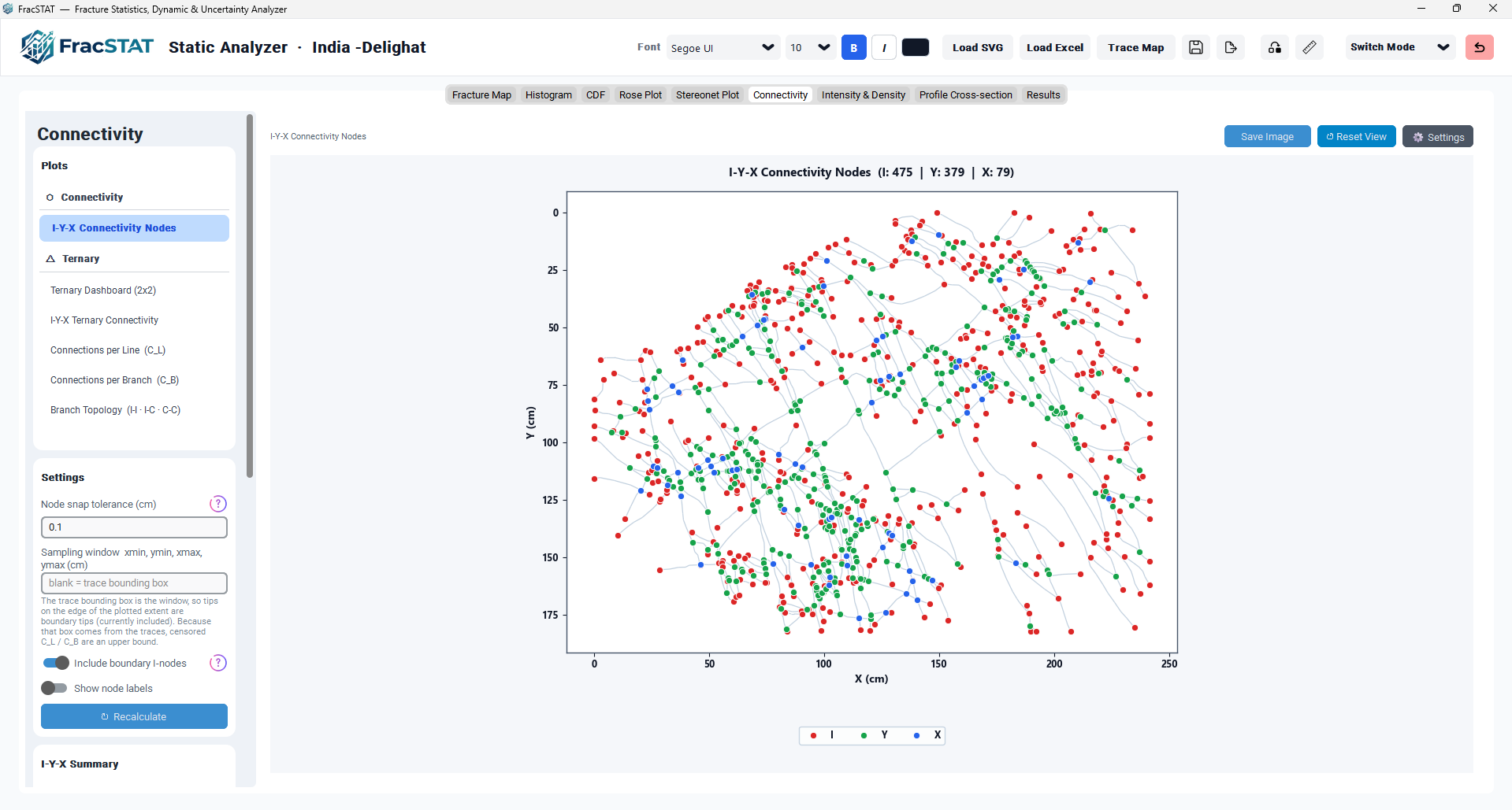
1.1 Sidebar Card Structure
| Card | Purpose |
|---|---|
| Plots | Grouped navigation buttons for switching between the six available diagrams (one Connectivity view, five Ternary views including the 2×2 dashboard). |
| Settings | Node snap tolerance entry, "Include boundary I-nodes" switch, "Show node labels" switch, and a Recalculate button. |
| I-Y-X Summary | Eight live numeric read-outs: I Nodes, Y Nodes, X Nodes, Total Nodes, Branches, Connected Fraction, Connections / Branch, B22. |
| Branch Topology | Five live numeric read-outs: I-I Branches, I-C Branches, C-C Branches, C_L, C_B. |
| Node Colours | A static colour legend explaining the three node-type colours used on the spatial map. |
1.2 Plot Navigation
The Plots card is organised into two labelled groups — Connectivity and Ternary. Clicking a
navigation button sets the active plot key, re-highlights the selected button (fill colour
changes to light blue, text turns bold and coloured), swaps the visible canvas via
grid()/grid_remove(), and updates the toolbar label above the plot.
Because all six Matplotlib canvases are constructed once at tab-build time and simply hidden
or shown, switching between diagrams is instantaneous and requires no recomputation.
| Group | Plot Key | Diagram |
|---|---|---|
| Connectivity | connectivity | I-Y-X Connectivity Nodes (spatial map) |
| Ternary | ternary_grid | Ternary Dashboard (2×2) — all four ternary diagrams below, laid out on a single canvas |
| Ternary | ternary_iyx | I-Y-X Ternary Connectivity |
| Ternary | ternary_cl | Connections per Line (C_L) |
| Ternary | ternary_cb | Connections per Branch (C_B) |
| Ternary | ternary_br | Branch Topology (I-I · I-C · C-C) |
1.3 Plot Area Toolbar
The toolbar above the plot canvas shows the name of the active diagram on the left and three action buttons on the right.
| Control | Action |
|---|---|
| ⬇ Save Image | Exports the currently active diagram to a timestamped PNG file inside the project's FracSTAT_plot_exports folder via the shared save_plot_image() helper. |
| ↺ Reset View | Restores the default pan/zoom extent of the active diagram without re-running the topological computation (recalculate=False). |
| ⚙ Settings | Toggles between the main sidebar and the Display Settings sidebar. |
2. Data Input
2.1 Upstream Data Source
The Connectivity tab does not load files directly. It consumes the same per-segment results
DataFrame (self.results) produced by the Static Analyzer's shared geometry engine
after an SVG or spatial Excel/CSV file is loaded, and reacts passively whenever results change
via the refresh_static_fluidflow() hook called from
StaticAnalyzerApp.refresh_all_tabs().
2.2 Required Columns
| Column | Description |
|---|---|
Trace | Integer or string identifier grouping segments belonging to the same digitised fracture trace. |
Segment | Integer identifier of a segment within its trace, used to order segments when extracting trace endpoints. |
X1, Y1, X2, Y2 | Real-world (scaled) coordinates of each segment's two endpoints, in the project's selected display unit (m, cm, mm, or km). |
2.3 Data-Source Gating
Before any computation is attempted, the tab checks whether the loaded data actually carries
genuine spatial geometry. SVG-digitised trace maps and spatial Excel/CSV imports are accepted.
Legacy orientation-only formats (ID/Strike/Dip tables, Trend/Plunge pole tables) are explicitly
rejected with an explanatory message — node counting on synthetic orientation-wheel coordinates
would be meaningless without real spatial position. The rejection test inspects whether the first
loaded Segment object carries a non-null _preset_strike attribute, set only by the
Excel loader for orientation-only formats.
2.4 Unit Handling
The tolerance entry field and all reported lengths and areas automatically track the project's
currently selected display unit (obtained from _static_map_unit_var, defaulting to
metres). The node-snap-tolerance label refreshes on every draw to show the active unit in
parentheses — e.g. "Node snap tolerance (m)" or "Node snap tolerance (cm)".
3. Settings and Controls
3.1 Settings Card (Main Sidebar)
| Control | Default | Effect |
|---|---|---|
| Node snap tolerance | 0.1 (display unit) | Distance threshold below which two nearby points are treated as the same physical node. Directly controls I/Y/X classification sensitivity. Committed on Enter or focus-loss; triggers a full recompute. |
| Sampling window xmin, ymin, xmax, ymax | Blank | The rectangular sample domain, entered as four numbers separated by commas, semicolons or spaces. It is a mathematical input, not a display setting: it defines the area A behind P20, P21, B₂₂ and P₂₂, and it is the rectangle that boundary I-nodes are measured against. Blank, unparseable, or degenerate (xmax ≤ xmin or ymax ≤ ymin) input falls back to the trace bounding box. Committed on Enter or focus-loss; forces a full recompute. |
| Include boundary I-nodes | Off (excluded) | When off and a sampling window has been entered, isolated (I) tips lying on the edge of that window are removed before counting — they are artefacts of the finite sample window rather than genuine fracture tips. When on, every I tip is retained. With no window entered the switch has no effect, because a boundary tip cannot be defined. Always forces a full recompute. |
| Show node labels | Off | Overlays a small text label (e.g. "I3", "Y12", "X1") beside every plotted node on the spatial map. Cosmetic only; does not trigger recomputation. |
| ↻ Recalculate | — | Forces an explicit, user-initiated recompute; shows the global loading overlay while the O(n²) intersection search runs. |
count_iyx_nodes(..., exclude_boundary_i=True); with the switch on, it calls
count_iyx_nodes(..., exclude_boundary_i=False). See
Section 5.4 for the extraction logic this parameter controls.
3.2 I-Y-X Summary Card
| Label | Symbol | Source |
|---|---|---|
| I Nodes | N_I | result.n_i — count of isolated fracture tips |
| Y Nodes | N_Y | result.n_y — count of abutting (T-shaped) intersections |
| X Nodes | N_X | result.n_x — count of crossing (X-shaped) intersections |
| Total Nodes | N | result.total_nodes = N_I + N_Y + N_X |
| Branches | N_B | result.branch_count = n_ii + n_ic + n_cc — the topological branch count from the trace walk (Section 5.7) |
| Connected Fraction | CF | result.connected_fraction = (N_Y + N_X) / N |
| Connections / Branch | C̄ | result.connections_per_branch = (3·N_Y + 4·N_X) / N_B, where N_B = (N_I + 3·N_Y + 4·N_X) / 2 — the node-derived count, so this equals C_B exactly |
| — | N_B (node form) | result.branch_count_from_nodes = (N_I + 3·N_Y + 4·N_X) / 2 — exposed for cross-checking against branch_count; not shown in the sidebar |
| B22 | B₂₂ | result.dimensionless_branch_intensity = L²_total / (A · N_B), with N_B = branch_count and A = sampling-window area |
3.3 Branch Topology Card
| Label | Symbol | Source |
|---|---|---|
| I-I Branches | N_II | result.n_ii — branches with both endpoints isolated |
| I-C Branches | N_IC | result.n_ic — branches with one isolated, one connected endpoint |
| C-C Branches | N_CC | result.n_cc — branches with both endpoints connected |
| C_L | C_L | Connections per line, recomputed locally in _update_branch_stats |
| C_B | C_B | Connections per branch, recomputed locally in _update_branch_stats |
3.4 Display Settings Sidebar
Clicking "⚙ Settings" hides the main sidebar and reveals a second sidebar of identical width, headed by a "⬅ Back" button and a title that reads either "Map Settings" or "Ternary Settings". The sidebar automatically swaps between two entirely independent panels depending on which diagram is currently active: the Map Settings panel is shown only while the spatial "I-Y-X Connectivity Nodes" plot is active, and the Ternary Settings panel is shown for all five Ternary-group plots (the dashboard and the four individual diagrams), which share one common set of controls. Every control in both panels is cosmetic and stylistic — none of them affect the underlying topological computation, only how the results are rendered. The two panels use separate colour/size variables under the hood, so styling the map does not affect the ternary diagrams and vice versa.
3.4.1 Map Settings — Plot Elements
| Control | Default | Effect |
|---|---|---|
| Outer background | theme background | Figure-level (canvas) background colour of the spatial map. |
| Plot background | theme panel | Axes-level background colour of the spatial map. |
| Grid colour | theme grid | Colour of the coordinate gridlines on the map. |
| I-Node colour | #DC2626 (red) | Marker colour for isolated nodes on the spatial map. |
| Y-Node colour | #16A34A (green) | Marker colour for abutting (Y) nodes on the spatial map. |
| X-Node colour | #2563EB (blue) | Marker colour for crossing (X) nodes on the spatial map. |
| Border colour | #475569 | Colour of the map's axis spines / plot border. |
| Border width | 1.0 | Line width (pt) of the map's axis spines. |
| Base Node Size | 36 | Base marker area (Matplotlib s parameter, in points²) for I, Y, and X node scatter markers on the spatial map. |
| Show scale | Off | Toggles a data‑accurate scale bar in the lower‑right of the spatial map, drawn in the project's current display unit. |
| Scale Color | #000000 | Colour used to draw the scale bar (and its label/ticks). |
| Scale style | Solid bar | Chooses how the scale bar is rendered — Solid bar (single filled block), Segmented bar (alternating filled/unfilled blocks), or Ticked line (a plain line with end ticks). |
| Show grid lines | Off | Toggles gridlines on the map. |
| Grid line width | 0.6 | Line width (pt) of the map's gridlines when shown. |
3.4.2 Map Settings — Background Image
| Control | Default | Effect |
|---|---|---|
| Show real photo behind nodes | Off | Enables a calibrated photograph drawn behind the spatial node map (the ternary diagrams do not use a background image). If no image path is yet known, automatically prompts a file browser or reuses an image already calibrated elsewhere in the project. |
| Change Image… | — | Opens a file dialog to (re)select the background photograph. |
| Image opacity (0–1) | 1.0 | Alpha blending factor applied to the background image via Matplotlib's imshow(alpha=...). |
3.4.3 Ternary Settings — Display Options
| Control | Default | Effect |
|---|---|---|
| Ternary plot heading | blank (automatic) | Custom title overriding the automatic heading on all five ternary diagrams (dashboard and individual views alike). |
3.4.4 Ternary Settings — Plot Elements
| Control | Default | Effect |
|---|---|---|
| Outer background | theme background | Figure-level (canvas) background colour of the ternary diagrams. |
| Plot background | theme panel | Axes-level background colour of the ternary diagrams. |
| Grid colour | theme grid | Colour of the ternary reference grid lines. |
| I-Node colour | #DC2626 (red) | Colour used for I-related vertex labels/markers on the ternary diagrams. |
| Y-Node colour | #16A34A (green) | Colour used for Y-related vertex labels/markers on the ternary diagrams. |
| X-Node colour | #2563EB (blue) | Colour used for X-related vertex labels/markers on the ternary diagrams. |
| Border colour | #475569 | Colour of the ternary axes' spines / plot borders. |
| Border width | 1.0 | Line width (pt) of the ternary axes' spines. |
| Show grid lines | Off | Toggles the ternary reference grid. |
| Grid line width | 0.6 | Line width (pt) of the ternary gridlines when shown. |
3.4.5 Ternary Settings — Grid & Axis Controls
| Control | Default | Effect |
|---|---|---|
| Grid interval | 0.2 | Spacing between reference gridlines on the ternary axes — a choice of 0.1, 0.2, or 0.25. |
| Grid line pattern | Dashed | Line style of the ternary reference grid — Solid, Dashed, Dotted, or Dash‑Dot. |
| Show edge tick marks | Off | Toggles small tick marks along the triangle's edges at each grid interval. |
| Tick direction | Outward | Draws the edge tick marks pointing Outward, Inward, or as a Cross through the edge. |
| Show edge labels | Off | Toggles numeric labels (e.g. "0.2", "0.4", …) alongside the edge tick marks. |
| Dashboard horizontal gap | 0.10 | Horizontal spacing (Matplotlib wspace) between the four subplots of the 2×2 Ternary Dashboard. |
| Dashboard vertical gap | 0.10 | Vertical spacing (Matplotlib hspace) between the four subplots of the 2×2 Ternary Dashboard. |
3.4.6 Ternary Settings — Data & Reference Elements
| Control | Default | Effect |
|---|---|---|
| Show point coordinates | Off | Annotates the observed data point on each ternary diagram with its raw coordinate values. |
| Marker style | — | Shape of the observed data point marker — Circle, Square, Triangle, or Diamond. |
| Marker size | — | Size of the observed data point marker. |
| Marker colour | — | Fill colour of the observed data point marker. |
| Marker border colour | — | Outline colour of the observed data point marker. |
| Marker border width | — | Outline thickness of the observed data point marker. |
| Show contour / locus lines | Off | Toggles the iso-value contour families (C_L, C_B) or the theoretical random-network locus (Branch Topology), depending on the active diagram. |
| Contour colour | — | Colour used to draw the contour / locus lines. |
| Show summary box | On | Toggles the small annotated text box (e.g. "C_L = 3.12") drawn on the C_L, C_B, and Branch Topology diagrams — see Section 3.4.7 for its drag behaviour. |
3.4.7 Interactive Dragging
When the workspace's "Move Layout Elements" edit mode is enabled, two figure annotations become click-and-draggable so they can be repositioned to avoid overlapping the underlying data:
| Element | Where it appears | Behaviour |
|---|---|---|
| Ternary summary box | C_L, C_B, and Branch Topology ternary diagrams | The annotated summary text (e.g. C_L, C_B value) can be dragged anywhere within its plot. Its position is tracked independently per diagram (cl, cb, br) and persists across redraws. |
| Map scale bar | Spatial connectivity map | When "Show scale" is enabled, the scale bar can be dragged to any position on the map; its anchor point is preserved across pan/zoom and redraw operations. |
Dragging either element suppresses the global "drag whole plot" pan handler for the duration of the drag, so repositioning an annotation never accidentally pans the underlying axes.
3.4.8 Reset Defaults
Because the Map Settings and Ternary Settings panels are independent, each has its own reset button, and only the button for the panel currently on screen is shown:
| Button | Shown when | Effect |
|---|---|---|
| Reset Map Defaults | Map Settings panel active | Restores every colour, size, and toggle in the Map Settings panel to its factory value and triggers a cosmetic-only redraw of the spatial map. Background-image settings are not affected. |
| Reset Ternary Defaults | Ternary Settings panel active | Restores every colour, size, and toggle in the Ternary Settings panel to its factory value and triggers a cosmetic-only redraw of the ternary diagrams. |
Neither button affects the underlying tolerance/boundary-inclusion settings that drive the topological computation.
4. Mathematical Background
Let S = {s₁, …, s_n} be the set of digitised segments, each defined by two endpoints (x1, y1) and (x2, y2) belonging to a parent trace.
4.1 Node Classes
Following the terminology introduced for fracture network topology (Manzocchi, 2002; Sanderson and Nixon, 2015), every distinct point where the network terminates or crosses itself is classified into exactly one of three mutually exclusive categories. The node names used here follow the standard fracture-network glossary (Peacock et al., 2016). The classification is a property of the trace, not of the individual straight segments a polyline happens to be digitised with: only the first point of a trace's first segment and the last point of its last segment are trace tips, and interior polyline vertices are never nodes.
| Symbol | Name | Geometric Definition | Branches | Geological Meaning |
|---|---|---|---|---|
| I | Isolated node | A trace tip that does not lie within snap tolerance of the interior of any other trace. | 1 | A fracture tip that terminates in intact rock — propagation stopped without linking to another fracture. |
| Y | Abutting node | A tip of one trace lying on the interior of another trace. | 3 | One fracture terminated against an earlier through-going fracture — the classic "T" intersection recording a relative age relationship. |
| X | Crossing node | Two trace interiors crossing, with the intersection point at a tip of neither trace. | 4 | Two fractures crossed each other, implying both were open/active at the time of intersection or that a younger fracture propagated straight through an older one. |
4.2 Node-Level Statistics
The connected fraction CF expresses what proportion of all identified nodes actually represent a connection between two or more fractures, as opposed to a dead end. It ranges from 0 (a network of entirely isolated fractures) to 1 (every node is a connection). The average connections per branch C̄ counts the total number of branch ends that terminate at Y- or X-nodes (3 per Y-node, 4 per X-node) and divides by the total number of branches N_B. Isolated I-nodes contribute only to the denominator, depressing C̄; a fully connected lattice with no I-nodes would approach the theoretical maximum C̄ = 2.
The identity N_B = (N_I + 3·N_Y + 4·N_X) / 2 is the node-degree relation of Sanderson and Nixon (2015, eq. 5): summing the branch ends meeting at every node counts each branch exactly twice. Because every node contributes an integer number of ends, the sum is always even and N_B is always an integer for a correctly classified network — a non-integer result is a diagnostic that some contact has been given the wrong node class.
result.branch_count is obtained by walking each trace and cutting it at its
nodes (Section 4.4); result.branch_count_from_nodes applies the
identity above to the node census. Their agreement is a genuine internal check on the node
classification. They diverge, legitimately, when boundary tips have been censored: the node
formula has no way to account for I nodes that were removed, so it under-counts relative to the
walked branch population. Note that connections_per_branch (C̄) divides by the
node-derived N_B, so C̄ and C_B in Section 4.5 are the same number by
construction, not two independent estimates.
4.3 Dimensionless Intensity (B₂₂ and P₂₂)
B₂₂ is the square of the cumulative trace length L_total, divided by the sample area A and
further normalised by the total branch count N_B, following
Sanderson and Nixon (2015, eq. 9).
It is a scale-independent measure of overall fracture density that can be compared directly
between outcrops of different sizes, and belongs to the same P₁₀/P₂₁/P₂₂ family of intensity
measures reviewed by Zhang and Einstein (2000).
ConnectivityResult also exposes a companion,
trace-normalised measure, P₂₂, computed the same way but dividing by the number of distinct
traces (trace_count) instead of the branch count. P₂₂ is available on the result
object for programmatic use but is not currently surfaced as a sidebar statistic in the
Connectivity tab.
N_B here is the topological branch count — trace portions between nodes — so B₂₂ does not change when a trace is re-digitised with more vertices. Substituting the raw segment count would make B₂₂ scale inversely with digitisation density and destroy comparability between hand-digitised and curve-sampled SVG traces.
The area A is the area of the sampling window. When a window is entered in the sidebar (Section 3.1) that window's area is used; otherwise A falls back to the bounding box of the digitised traces, which makes B₂₂ and P₂₂ conditional on the traces themselves rather than on an independently chosen sample domain.
4.4 Branch Classification
A branch is the portion of a trace between two nodes. It is not the same thing as a digitised segment: an isolated trace drawn with one straight segment and the same trace drawn with fifty both contain exactly one branch. The module therefore walks each trace in digitised order and cuts it only where a node falls — at an X or Y node inside a segment, or at an interior polyline vertex that happens to coincide with a node. Interior vertices that are not nodes never cut. Each resulting branch has its two ends tested for proximity to the accepted X∪Y node set and labelled C (connected) or I (isolated):
| Class | End Pattern | Symbol | Meaning |
|---|---|---|---|
| I–I | isolated – isolated | n_ii | A fully isolated strand that neither terminates against nor is crossed by any other fracture at either end. |
| I–C | isolated – connected | n_ic | A branch that dangles freely at one end but connects to the network at the other — a "dead-end spur". |
| C–C | connected – connected | n_cc | A branch connected to the rest of the network at both ends — the fully connected, fluid-conducting portion of the fracture set. |
This walked census is the value reported as result.branch_count and used in B₂₂. It
is cross-checked against the node-derived count of Section 4.2.
4.5 Line- and Branch-Density Ratios (C_L and C_B)
N_L is an estimate of the number of discrete "lines" (through-going fracture traces) implied by
the node population, and C_L (connections per line) expresses how many connections, on average,
each such line participates in. N_Br applies the node-degree identity of
Section 4.2, so C_B is numerically identical to the
connections_per_branch property; the independent cross-check on the branch
population is branch_count from the trace walk, not C_B.
4.6 Ternary (Barycentric) Coordinates
Each of the four ternary diagrams plots a data point inside an equilateral triangle using standard barycentric-to-Cartesian conversion. For any three proportions p_bl, p_br, p_apex that sum to 1, the Cartesian plotting position within a unit-height triangle is:
For the I-Y-X ternary, the vertex assignment is bottom-left = Y fraction, bottom-right = X fraction, apex = I fraction (i.e. p_i = N_I/N, p_y = N_Y/N, p_x = N_X/N). For the Branch Topology ternary, the three proportions are the I-I, I-C, and C-C branch fractions: p_ii at the apex, p_cc at bottom-right, p_ic at bottom-left.
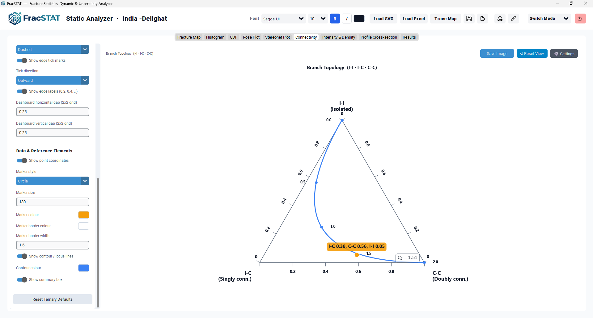
4.7 Theoretical Random-Network Locus (Branch Topology Ternary)
The Branch Topology diagram overlays a reference curve corresponding to the theoretical relationship expected for a network where node connectivity follows a simple binomial (random) model. Parameterising by C_B ∈ [0, 2] and setting p_C = C_B / 2:
The locus is plotted as a smooth blue curve with tick marks at C_B = 0.0, 0.5, 1.0, 1.5, 2.0, giving the analyst an immediate visual reference for how far the observed network departs from a purely random connectivity structure. Real fracture networks are typically displaced toward the C-C corner relative to this random-model curve (Sanderson and Nixon, 2018).
5. Algorithms
The complete node-classification and branch-typing pipeline is implemented in
core/branch_counter.py, function count_iyx_nodes(), and is called
from the GUI layer only when a recompute is actually required (Section 10).
5.1 Pre-processing and Validation
If the results table is empty or missing any of the required geometry columns (Trace, Segment,
X1, Y1, X2, Y2), the function immediately returns an all-zero
ConnectivityResult. All coordinate columns are coerced to numeric
(pandas.to_numeric, errors='coerce'); rows that fail conversion are dropped.
Segments shorter than 1×10⁻¹² are discarded as degenerate. The tolerance is clamped to be
non-negative (max(tolerance, 0.0)). Two rectangles are then established: the
bounding box of the surviving coordinates (data_bounds), and the reported sampling
window (bounds), which is the caller-supplied sample_bounds when one is
given and otherwise falls back to data_bounds. The reported window anchors both the
boundary-exclusion test and the sample area A used by B₂₂ and P₂₂.
A per-trace tip lookup is also built by _trace_tip_lookup(), mapping each trace to
the two coordinates that are genuinely its tips. This is what makes the node classification in
Section 5.3 a trace-level rather than a segment-level test.
5.2 Pairwise Segment Intersection
For every distinct pair of segments belonging to different traces (segments sharing the same Trace identifier are never tested against each other), the module solves the standard 2-D parametric line intersection system:
The tolerance is converted from an absolute map distance into a fractional parametric extension (tol_a = tol / L₁, tol_b = tol / L₂) so that the snap distance scales correctly with segment length. The accepted point is then computed by substitution back into the first segment's parametric equation, with ua and ub clamped to [0, 1].
5.3 Classifying the Intersection: Abutment vs Crossing
Each accepted intersection is tested against the tips of the parent traces, not against
the endpoints of the two segments that happened to intersect. _at_trace_tip()
compares the intersection point, by Euclidean distance under the user-specified tolerance,
against the two tips of trace i and then against the two tips of trace j. This
yields two booleans — tip_i and tip_j — and the classification follows
a four-way decision table:
| tip_i | tip_j | Node class | Splits recorded |
|---|---|---|---|
| True | True | none — 2-branch tip-to-tip contact; both tips stay I nodes | none |
| True | False | Y (trace i abuts trace j) | segment j at ub |
| False | True | Y (trace j abuts trace i) | segment i at ua |
| False | False | X (two trace interiors cross) | both segments at their respective u-values |
Testing segment endpoints instead would call an interior polyline vertex a trace tip and so
downgrade a genuine 4-branch crossing to a 3-branch Y node — an error that grows with
digitisation density, because the denser a polyline is sampled the more interior vertices there
are to be mistaken for tips. Splits are recorded whenever the relevant clamped parametric
coordinate lies strictly inside (0, 1); those coordinates populate the per-segment
seg_splits table used for the branch walk.
5.4 Trace-Tip (I-node) Extraction and Boundary Exclusion
Independently of the pairwise intersection search, the true tips of every trace are
extracted by _trace_endpoints(): segments are grouped by Trace and sorted by
Segment, and the first coordinate of the first segment and the second coordinate of the last
segment in each trace are taken as the two trace-tip candidates — correctly handling
multi-segment traces even though the trace is stored as a chain of individual straight segments.
I nodes are counted per trace tip, not per unique location. Because
_trace_endpoints() already emits exactly two points per trace there are no
floating-point duplicates to merge, and no clustering is applied to them. Clustering here would
collapse the two distinct tips of a tip-to-tip contact into a single node, and the branch-end
bookkeeping would break: N_B = (N_I + 3·N_Y + 4·N_X) / 2 would stop being an integer. Each tip
contributes exactly one branch end.
If "Include boundary I-nodes" is off (the default) and a sampling window has been
supplied, every candidate tip lying within tolerance of a side of that window is discarded by
_on_boundary(). This censoring correction reflects the fact that a trace exiting
the mapped area is not truly an isolated fracture tip — it is an artefact of the finite sample
window.
exclude_boundary_i is honoured only when sample_bounds is
supplied; with no window the switch has no effect and every tip is retained.
5.5 Point Clustering
Because floating-point intersection arithmetic can produce several near-duplicate points
representing the same physical intersection, the raw X and Y candidate sets are merged by
_cluster_points() using a greedy single-pass
algorithm: each new candidate point is compared, in the order encountered, against the running
centroid of every cluster created so far. If it lies within tolerance of an existing cluster
centroid, it is merged and the centroid is updated as the incremental running mean; otherwise a
new cluster is started. As noted in Section 5.4, I-node candidates are
deliberately excluded from this step.
5.6 Priority-Ordered De-duplication Across Classes
After clustering, three independent point sets exist. Any Y candidate also matching an X cluster
is removed via _remove_points_near() (a true crossing takes priority over a
coincidental abutment). Any I candidate matching an X or Y cluster is removed (a genuine
intersection always takes priority over an apparent near-miss tip). This produces the
strict, mutually exclusive priority ordering X > Y > I, ensuring every physical location
is counted exactly once in its most topologically significant category.
5.7 The Branch Walk and Classification
The final stage (_classify_branches) counts branches by walking each
trace, not by subdividing each segment. Segment rows are grouped by Trace and
ordered by Segment so the walk follows the trace as digitised. For each trace an ordered list of
cut points is assembled from two sources: every X/Y node recorded in seg_splits that
falls inside one of its segments, and any interior polyline vertex that itself coincides with a
node. Interior vertices that are not nodes never cut, which is what makes the branch count
independent of digitisation density.
The trace's own start and end are then prepended and appended, consecutive points closer than the
tolerance are collapsed, and each consecutive pair defines one branch. Both of its ends are
tested against the merged X∪Y node set by is_connected() and the branch is assigned
to the I-I, I-C or C-C class. A trace with no cuts contributes exactly one branch.
def count_iyx_nodes(results, tolerance=1.0, exclude_boundary_i=True,
                    progress_callback=None, sample_bounds=None):
    """Classify I/Y/X nodes and I-I/I-C/C-C branches from spatial trace data.

    Nodes are classified by TRACE-level topology (Sanderson & Nixon 2015):
    I = isolated trace tip (1 branch), Y = a tip abutting another trace's
    interior (3 branches), X = two trace interiors crossing (4 branches).
    Two tips that merely touch form a 2-branch contact, which is none of
    I/Y/X; both tips stay I nodes.

    ``sample_bounds`` is the independently defined sampling window
    (xmin, ymin, xmax, ymax).  ``exclude_boundary_i`` is honoured only when
    it is supplied, because boundary tips cannot be identified against a
    window derived from the traces themselves.
    """
    if results is None or results.empty:
        return _empty_result()

    cols = ("Trace", "Segment", "X1", "Y1", "X2", "Y2")
    missing = [c for c in cols if c not in results.columns]
    if missing:
        raise ValueError(f"Missing geometry column(s): {', '.join(missing)}")

    segs = results[list(cols)].copy()
    for col in ("X1", "Y1", "X2", "Y2"):
        segs[col] = pd.to_numeric(segs[col], errors="coerce")
    segs = segs.dropna(subset=["X1", "Y1", "X2", "Y2"])

    xy = segs[["X1", "Y1", "X2", "Y2"]].to_numpy(dtype=float)
    traces = segs["Trace"].to_numpy()
    lengths = np.hypot(xy[:, 2] - xy[:, 0], xy[:, 3] - xy[:, 1])
    valid = lengths > 1e-12
    xy, traces, segs, lengths = xy[valid], traces[valid], segs.iloc[np.nonzero(valid)[0]], lengths[valid]

    tol = max(float(tolerance), 0.0)
    xs, ys = np.concatenate([xy[:, 0], xy[:, 2]]), np.concatenate([xy[:, 1], xy[:, 3]])
    data_bounds = (float(xs.min()), float(ys.min()), float(xs.max()), float(ys.max()))

    # The reported window is the caller's sampling window when one is known;
    # otherwise it falls back to the data extent, which makes every intensity
    # measure conditional on the traces themselves.
    bounds = tuple(float(v) for v in sample_bounds) if sample_bounds is not None else data_bounds
    sample_area = max((bounds[2] - bounds[0]) * (bounds[3] - bounds[1]), 0.0)

    segment_order = segs["Segment"].to_numpy()
    trace_tips = _trace_tip_lookup(segs)          # trace id -> its two TIPS

    x_candidates, y_candidates = [], []
    seg_splits = defaultdict(list)

    # Pairwise intersection search (O(n^2), cross-trace pairs only)
    for i in range(len(xy)):
        for j in range(i + 1, len(xy)):
            if traces[i] == traces[j]:
                continue
            hit = _segment_intersection(xy[i], xy[j], tol)
            if hit is None:
                continue
            x, y, ua, ub = hit

            # Topology is a property of the TRACE, not of the arbitrary segment
            # a polyline happens to be broken into.
            tip_i = _at_trace_tip(x, y, trace_tips.get(traces[i]), tol)
            tip_j = _at_trace_tip(x, y, trace_tips.get(traces[j]), tol)

            if tip_i and tip_j:
                continue                      # 2-branch contact: both stay I
            if tip_i and not tip_j:
                y_candidates.append((x, y))
                if 0.0 < ub < 1.0:
                    seg_splits[j].append((ub, x, y))
            elif tip_j and not tip_i:
                y_candidates.append((x, y))
                if 0.0 < ua < 1.0:
                    seg_splits[i].append((ua, x, y))
            else:
                x_candidates.append((x, y))   # two trace interiors cross
                if 0.0 < ua < 1.0:
                    seg_splits[i].append((ua, x, y))
                if 0.0 < ub < 1.0:
                    seg_splits[j].append((ub, x, y))

    # Cluster X and Y only, then de-duplicate with priority X > Y > I
    x_nodes = _cluster_points(x_candidates, tol)
    y_nodes = _remove_points_near(_cluster_points(y_candidates, tol), x_nodes, tol)

    endpoint_candidates = _trace_endpoints(segs)
    if exclude_boundary_i and sample_bounds is not None:
        endpoint_candidates = [p for p in endpoint_candidates
                               if not _on_boundary(p, bounds, tol)]

    # I nodes are counted per TRACE TIP, not per unique location: clustering
    # here would merge the two tips of a tip-to-tip contact into one node and
    # N_B = (N_I + 3*N_Y + 4*N_X)/2 would stop being an integer.
    i_nodes = (np.asarray(endpoint_candidates, dtype=float)
               if endpoint_candidates else np.empty((0, 2), dtype=float))
    i_nodes = _remove_points_near(i_nodes, x_nodes, tol)
    i_nodes = _remove_points_near(i_nodes, y_nodes, tol)

    # Branches counted by walking each trace and cutting only at its nodes
    n_ii, n_ic, n_cc = _classify_branches(
        xy, traces, segment_order, x_nodes, y_nodes, tol, seg_splits
    )
    branch_count = n_ii + n_ic + n_cc

    return ConnectivityResult(
        i_nodes=i_nodes, y_nodes=y_nodes, x_nodes=x_nodes,
        bounds=bounds, trace_count=int(pd.Series(traces).nunique()),
        segment_count=int(len(xy)), branch_count=branch_count,
        total_length=float(lengths.sum()), sample_area=float(sample_area),
        n_ii=n_ii, n_ic=n_ic, n_cc=n_cc,
    )
5.8 Algorithm Complexity Summary
| Stage | Complexity | Notes |
|---|---|---|
| Pairwise intersection search (first pass) | O(n²) | n = number of segments; every cross-trace pair is tested once. |
| Point clustering | O(k²) per class | k = raw candidate count for X or Y, typically ≪ n². I-node candidates are not clustered. |
| Trace-tip lookup | O(n log n) | One sort of the segment table by (Trace, Segment); two tip coordinates stored per trace. |
| Boundary exclusion | O(m) | m = number of trace-tip candidates (2 per trace). Skipped entirely when no sampling window is supplied. |
| Branch walk & classify | O(n · s) | s = cuts per segment; uses seg_splits accumulated during the first pass, so no repeated O(n²) intersection search. |
The dominant cost is quadratic in the number of segments. For very dense SVG traces (many thousands of short curve-sampled segments), this can become the single most expensive computation in the entire Static Analyzer workspace.
6. Statistical Methods
Unlike the Histogram or CDF tabs, the Connectivity module does not perform inferential statistics. Its statistical content is entirely descriptive and topological: it counts, classifies, and ratios discrete network elements. All reported quantities are deterministic functions of the digitised geometry and the three user-controlled parameters (snap tolerance, sampling window, boundary-I-node inclusion). No sampling error or estimator variance is associated with these numbers in the classical statistical sense.
| Quantity | Type | Range | Interpretation |
|---|---|---|---|
| N_I, N_Y, N_X | Count (integer) | ≥ 0 | Absolute abundance of each node class. |
| N (total nodes) | Count (integer) | ≥ 0 | Sum of all node classes. |
| Connected Fraction CF | Proportion | [0, 1] | Higher = more of the network participates in genuine connections rather than dead ends. |
| Connections / Branch C̄ | Ratio (dimensionless) | ≥ 0 | Average branch-end connectivity, weighted 1× for Y and 2× for X. |
| B₂₂ | Dimensionless intensity | ≥ 0 | Scale-independent overall fracture density (P₂₂-style intensity metric). |
| N_II, N_IC, N_CC | Count (integer) | ≥ 0 | Branch population by connectivity class. |
| C_L | Ratio (dimensionless) | typically 0–4 | Connections per fracture line. |
| C_B | Ratio (dimensionless) | typically 0–2 | Connections per branch; theoretical random-network bound is exactly 2. |
| Barycentric ternary position | Composition (proportion triple) | simplex | Visual, compositional summary of any of the three-part classifications above. |
The principal sources of uncertainty are (a) digitisation error in the original trace map, (b) sensitivity to the chosen snap tolerance, and (c) truncation/censoring at the edges of the mapped domain. None of the three is propagated into a reported confidence interval, so the recommended practice is a sensitivity sweep: recompute the node census at two or three snap tolerances and report the spread. The same node-counting definitions are implemented in the established open fracture-network toolboxes (Healy et al., 2017; Nyberg et al., 2018), so counts from this tab are directly comparable with theirs provided the tolerance and window are matched.
7. Visualization & Figure Components
Six selectable Matplotlib diagrams are available, switchable instantly from the Plots
navigation card. All share the workspace's global font-size, font-weight, and font-colour
settings (matplotlib.rcParams), and each honours the Display Settings colour/size
overrides for its own family — the spatial map reads the Map Settings panel, and the four
ternary diagrams plus the dashboard all read the shared Ternary Settings panel — described in
Section 3.4.
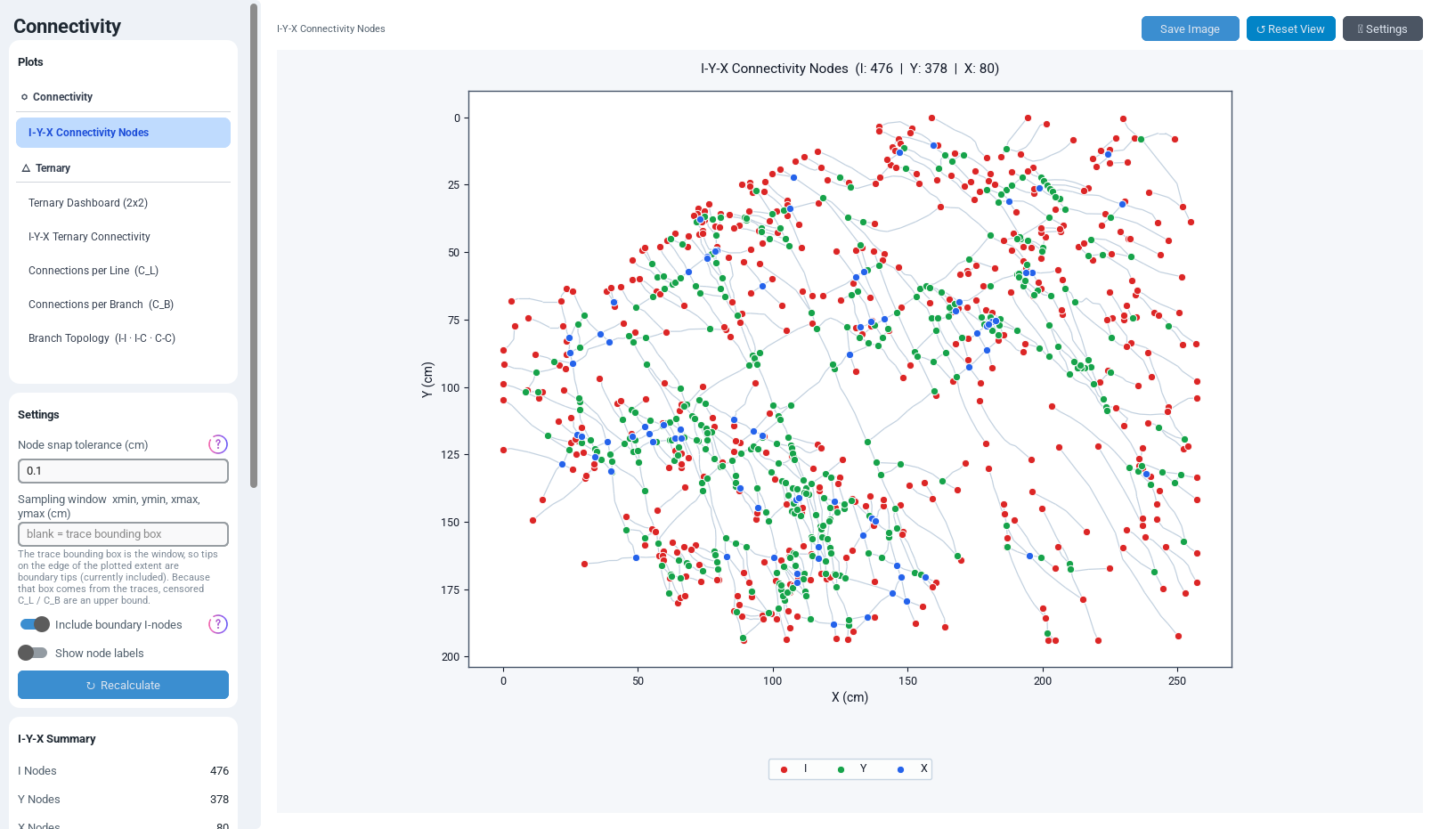
7.1 I-Y-X Connectivity Nodes (Spatial Map)
This is the only diagram drawn in true map (X, Y) coordinates. Every digitised segment is
rendered as a thin line (LineCollection, using the theme's spine/border colour),
and the three node classes are overlaid as coloured scatter points: red for I, green for Y,
blue for X by default. Marker size follows the "Base Node Size" setting. If "Show node
labels" is enabled, each node receives a small text label (e.g. "X7") numbering it within its
class. A legend with three columns is drawn beneath the plot. The axes are scaled equal (1:1
aspect) and padded by 5% of the bounding-box extent on each side.
7.2 Ternary Dashboard (2×2)
Selected via the ternary_grid plot key, this diagram draws all four ternary plots
described in Sections 7.3–7.6 together as a single 2×2 grid of subplots on one canvas, so the
full ternary picture — connectivity, C_L, C_B, and Branch Topology — can be compared at a
glance without switching between individual views. Each subplot is drawn with the same
routine used for its full-size counterpart, so any Ternary Settings change (colours, grid,
markers, contours) applies identically to the dashboard and to the individual diagrams. The
spacing between the four subplots is controlled independently via the "Dashboard horizontal
gap" and "Dashboard vertical gap" settings (see Section 3.4.5).
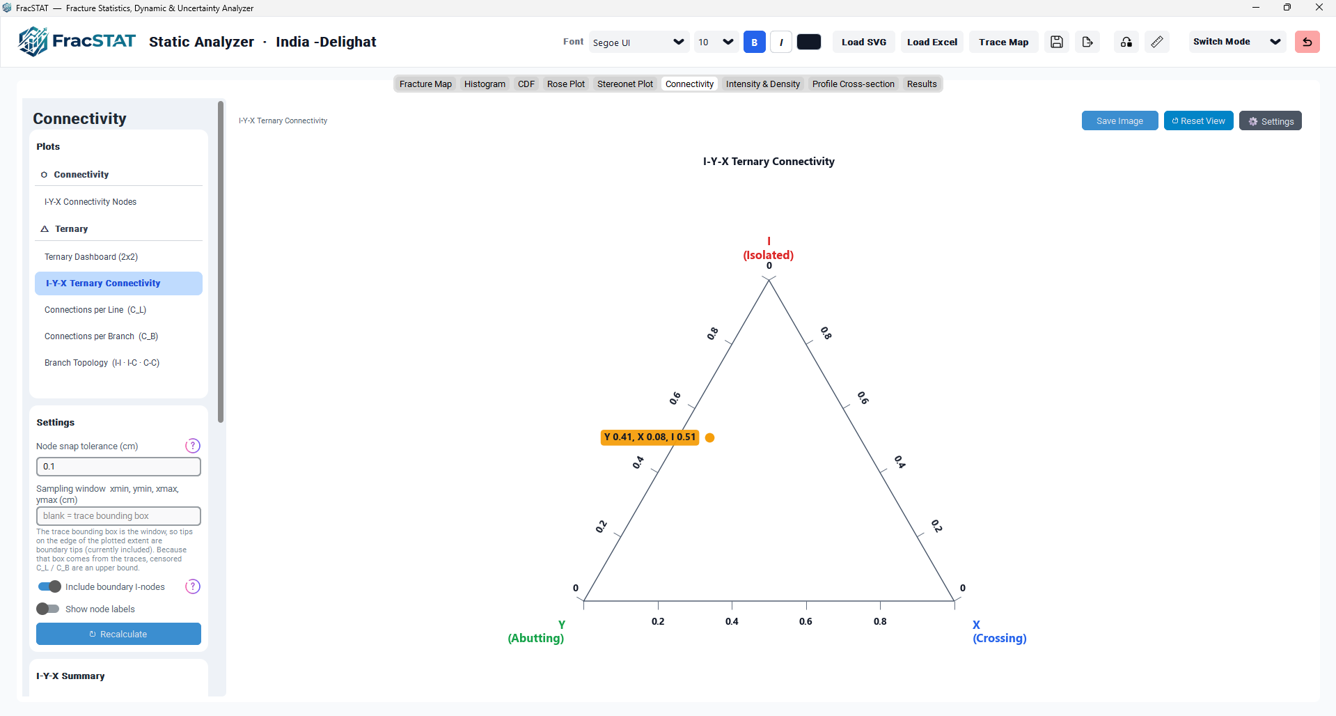
7.3 I-Y-X Ternary Connectivity
An equilateral-triangle ternary diagram with vertices labelled Y (bottom-left), X (bottom-right), and I (apex). A single orange marker plots the network's (p_i, p_y, p_x) composition using the barycentric transform of Section 4.6, annotated with a text callout reporting all three fractions to two decimal places (e.g. "I 0.32 Y 0.41 X 0.27"). A point sitting close to the Y-X base edge indicates a well-connected network dominated by terminations and crossings rather than dead ends.
7.4 Connections per Line (C_L)
The same Y/X/I ternary frame, overlaid with a family of iso-C_L contour lines drawn for C_L = 1, 2, 3, 4, 6, 8, 10, 20, plus a distinguished dashed contour at the frequently cited threshold C_L = 3.57 — the value associated with the transition to well-connected, likely- percolating networks in several published topological classifications. The observed data point is plotted as an amber marker with an annotated C_L value.
7.5 Connections per Branch (C_B)
Structurally identical to the C_L diagram but contoured for C_B = 0.5, 1.0, 1.3, 1.5, 1.7, 1.8, 1.9, 1.95, plus the fixed C_B = 2.0 contour, which coincides exactly with the bottom (Y–X) edge of the triangle since C_B = 2 is the theoretical maximum (every branch fully connected at both ends, i.e. zero I-nodes). The observed point is plotted as a cyan marker with an annotated C_B value.
7.6 Branch Topology (I-I · I-C · C-C)
A ternary diagram with vertices I-C (bottom-left), C-C (bottom-right), and I-I (apex), overlaid with the theoretical random-network locus described in Section 4.7 (blue curve with C_B tick labels at 0.0–2.0) and the observed branch-population point plotted as a white marker with a dark outline, annotated with its independently computed C_B value derived from the I-I/I-C/C-C proportions.
7.7 Empty and Loading States
When no data is loaded, when the data source lacks real map geometry, or while a recomputation
is pending but the tab is not the active one, all six axes are cleared and a single centred,
muted-colour text message is drawn by _fluid_empty_state() explaining the reason.
All sidebar statistic labels are simultaneously reset to "–".
7.8 Global Styling Controls
The spatial map and the ternary diagrams each observe their own independent set of
background/foreground/grid/border colour variables and their own border line width and grid
line width entries (see Section 3.4), so the two families can be styled
completely independently. Within a family, though, every diagram shares one consistent,
publication-ready style suite — the four individual ternary diagrams and the 2×2 dashboard all
read the same Ternary Settings. Corner labels and axis titles automatically scale with the
workspace's global font-size control (mpl.rcParams['axes.titlesize']).
8. Step-by-Step Example Workflows
8.1 Assessing Reservoir Connectivity from an Outcrop Trace Map
- Load an SVG trace map (or a spatial Excel/CSV) into the Static Analyzer and confirm the Fracture Map tab renders correctly with calibrated scale.
- Open the Connectivity tab. Because the data is new, the tab is marked stale and an automatic lazy computation runs immediately with the default 0.1-unit tolerance.
- Inspect the I-Y-X Connectivity Nodes map. Visually confirm that crossing (blue) markers sit at genuine X-shaped intersections, and abutting (green) markers at T-shaped terminations. If many genuinely touching fracture tips are coloured red (I), the snap tolerance is too small relative to digitisation precision; if unrelated nearby fractures are merged into a single node, the tolerance is too large.
- Adjust "Node snap tolerance" as needed (e.g. from 0.1 m to 0.25 m for coarse digitisation) and press "↻ Recalculate".
- Decide on boundary I-nodes: use exclusion (the default) for an arbitrary rectangular crop of a larger fracture field; use inclusion if fracture tips genuinely terminate at a natural geological boundary such as a bounding fault.
- Read the I-Y-X Summary card: for example, I = 42, Y = 118, X = 76, Total = 236, Branches = 310, CF = 0.822, C̄ = 0.877, B₂₂ = 4.6.
- Switch to the I-Y-X Ternary diagram — a point sitting close to the Y-X edge (away from the I apex) indicates a well-connected network.
- Switch to the C_L diagram — a point to the right of the dashed C_L = 3.57 contour indicates a topologically well-connected, likely-percolating regime.
- Switch to the Branch Topology diagram — a point displaced toward the C-C corner relative to the random-network locus suggests connectivity in excess of a purely random linking process, consistent with mechanically controlled fracture growth.
- Use "⬇ Save Image" on each diagram of interest to export 300 dpi PNGs to the project's
FracSTAT_plot_exportsfolder for inclusion in a report or publication.
8.2 Worked Numerical Example
Consider a network reporting I = 10, Y = 20, X = 10 (N = 40 nodes). The node census fixes the branch population before any branch is walked: the branch ends sum to 10·1 + 20·3 + 10·4 = 110, so N_B = 110 / 2 = 55. Ten of those ends are isolated, so the walked census must satisfy 2·N_II + N_IC = 10 and N_II + N_IC + N_CC = 55 — for instance N_II = 0, N_IC = 10, N_CC = 45. The connectivity statistics are:
The agreement between 55 and 0 + 10 + 45 is the check worth performing on real data. A mismatch means either that boundary tips were censored — in which case the node formula legitimately under-counts, because the removed I nodes are missing from it — or that a contact has been given the wrong node class. A non-integer N_B is always the second case.
With C_B = 1.82 exceeding the well-connected reference value of 1.7–1.8 commonly cited in topological classifications, and C_L = 4.0 exceeding the 3.57 percolation-related threshold, this hypothetical network would be characterised as well connected and likely to behave as an effective fluid-flow pathway network.
9. Geological Interpretation
9.1 Connectivity Statistics and Fluid Flow
Fracture connectivity, not fracture density alone, is frequently the controlling factor in whether a naturally fractured reservoir, aquifer, or rock mass behaves as an effective flow or mechanical system (National Research Council, 1996). Two intervals with identical fracture intensity (P10, P21, or B₂₂) can have dramatically different bulk permeability if one is dominated by isolated fractures (high I-node fraction, low CF) while the other forms an interconnected lattice (high X/Y-node fraction, high CF) — the classic result that effective permeability rises steeply with the degree of interconnection rather than with fracture abundance (Long and Witherspoon, 1985; Odling et al., 1999).
9.2 Node-Type Ratios and Network Maturity
Increasing abundance of crossing (X) nodes relative to abutting (Y) nodes is often associated with a more mature, multiply-reactivated fracture system where successive fracture sets have propagated through pre-existing fractures rather than systematically terminating against them. Conversely, a network dominated by Y-nodes frequently records a clear relative-age sequence, with younger, shorter fractures terminating against an earlier, more continuous fracture set — a pattern common in systematically jointed sedimentary sequences with a dominant bedding-perpendicular joint set.
9.3 Percolation and Effective Connectivity Thresholds
The C_L = 3.57 and C_B ≈ 2 reference values on the ternary diagrams derive from topological and percolation-theory studies of two-dimensional fracture networks (Robinson, 1983; Berkowitz, 1995; Sanderson and Nixon, 2018), where networks below the threshold are statistically unlikely to form a fully connected percolating cluster spanning the sample domain, while networks above typically do. These are heuristic reference values rather than universal physical constants: the true percolation threshold for any specific network depends on the fracture-length distribution, orientation distribution, and aperture/permeability contrast, quantified separately in other FracSTAT tabs. Spatial correlation between fractures shifts the threshold further still (Manzocchi, 2002).
9.4 Dead-End Branches (I-C) and Hydraulic Significance
A large I-C (dead-end spur) fraction indicates that a substantial portion of the mapped fracture length — while nominally connected to the main network at one end — terminates in intact rock at the other and cannot itself provide a through-going flow path. Distinguishing the C-C (fully connected, potentially conductive) branch population from the I-C and I-I populations is therefore directly relevant when the Connectivity results are combined with permeability up-scaling or discrete-fracture-network flow simulation performed outside FracSTAT.
9.5 Scale Dependence and Sampling Considerations
Connectivity statistics are not fully scale-invariant: the observed I-node fraction is sensitive to the size of the mapped domain relative to the mean fracture length, because a larger domain captures more complete fracture traces (fewer artificial edge terminations). The boundary-I-node exclusion option partially corrects for this effect, but only when a sampling window has been entered — it is the window edge that defines an artificial termination. Analysts should still be cautious when comparing connectivity statistics computed from maps of substantially different physical size or aspect ratio (Watkins et al., 2015). Where an unbiased, edge-effect-free intensity estimate is the objective, the circular-window and circular-scanline estimators (Mauldon et al., 2001) are the established alternative to a rectangular window; they are not implemented in this tab.
10. Performance Optimization
Because the underlying topological computation is O(n²) in the number of digitised segments, the Connectivity tab is deliberately engineered to run this computation as rarely as possible while still guaranteeing that displayed statistics are always correct and current.
10.1 Result Caching
The single ConnectivityResult object produced by the most recent successful call
to count_iyx_nodes() is retained in self._fluid_connectivity for
the lifetime of the workspace session. Every cosmetic redraw (colour change, grid toggle,
node-label toggle, pan, zoom, Reset View) reuses this cached object directly rather than
recomputing it.
10.2 Lazy, On-Demand Computation
The tab is only ever computed when it is both (a) marked stale by a genuine geometry change and (b) actually the currently visible tab (or explicitly forced via Recalculate or a settings change that mandates recomputation). If the analyst never opens the Connectivity tab, the expensive computation never runs at all, regardless of how many files are loaded or how many times the profile scale is changed elsewhere in the workspace.
10.3 Geometric Fingerprinting
Every time refresh_static_fluidflow() is called, it computes a cheap fingerprint
of the current results table — the tuple (row count, rounded total segment length). The
fingerprint is O(1) to compare and O(n) to compute, several orders of magnitude cheaper than
the O(n²) computation it guards. It changes only when the underlying digitised geometry itself
has changed, remaining completely insensitive to purely cosmetic changes such as colour, font,
or grid visibility.
10.4 Deferred Execution and UI Responsiveness
Because the algorithm can take perceptible wall-clock time for dense digitisations, every user
action that may trigger a recompute is scheduled through Qt's after(100, …)
mechanism rather than executed synchronously. This 100 ms delay is sufficient for the global
loading overlay to be physically painted to the screen before the main thread blocks on the
O(n²) search, so the application never appears to freeze without explanation.
10.5 Single-Figure-per-Diagram Construction
All five Matplotlib Figure/Axes/Canvas triples are constructed exactly once at tab-build time and simply shown/hidden thereafter. This avoids the overhead of destroying and rebuilding Matplotlib canvases every time the analyst switches between the five available diagrams, at the modest cost of holding five figures in memory simultaneously.
10.6a Session Restore Behaviour
Restoring a saved session sets the active tab via tabs.set(), which does not fire
the same tab-click handler that normally triggers a draw when the analyst manually switches to
the Connectivity tab. To prevent the diagrams from appearing blank until the analyst clicks
away and back, refresh_static_fluidflow() now checks whether a cached
ConnectivityResult already exists for a non-stale, non-active Connectivity tab and,
if so, draws it immediately (recalculate=False) so the plots are ready the instant
the tab is opened.
10.6 Recommended Practice for Large Data Sets
For SVG traces exceeding several thousand segments, consider increasing the Curve step (px) parameter when loading the SVG to reduce the number of straight-line segments used to approximate curved traces. Adjust the snap tolerance thoughtfully before pressing Recalculate rather than repeatedly nudging it — each change re-triggers the full O(n²) computation. Leave "Show node labels" off for very dense networks, as densely overlapping text labels can noticeably slow down canvas rendering and obscure the spatial map.
11. Advanced Features
11.1 Interactive Pan and Zoom
All five canvases share a common pair of mouse-driven navigation handlers connected at
tab-build time. The scroll wheel (_on_scroll_zoom) zooms in or out by a fixed
1.2× factor per click, centred exactly on the cursor position so that the data-space
coordinate under the cursor is held fixed while the axis limits are rescaled around it.
Left-click drag (_on_mouse_press / _on_mouse_drag /
_on_mouse_release) pans the active diagram by translating both axis limits by the
same data-space displacement as the cursor. "↺ Reset View" restores the default extent
without any recomputation.
11.2 Custom Colour Picker
Every colour swatch in the Display Settings sidebar opens the shared FracSTAT colour-picker
dialog (_StaticColorButton), which presents a curated 8×5 matrix of 40
professionally chosen preset swatches spanning eight hue families at five lightness levels,
plus a free-form hex-code entry field with a live preview patch. Selecting a preset or typing
a valid hex code and pressing "Apply" immediately re-fires the connectivity redraw callback
bound to that colour variable.
11.3 Calibrated Background Photograph Overlay
The Connectivity tab supports overlaying a real, scale-calibrated photograph of the outcrop
behind the spatial node map (the four ternary diagrams do not use a background image). The
implementation (_autodetect_fluid_bg_image_path()) searches in priority order:
(1) an image path already stored in this tab's own StringVar; (2) the Fracture Map tab's own
calibrated background image variable, if set; (3) a sidecar PNG automatically saved alongside
a traced SVG by the Trace Map tool (named <svg-basename>_bg.png). The
chosen path is cached in memory so repeated redraws do not re-read the file from disk. The
image is drawn with imshow, its extent locked to the bounding box of the current
fracture geometry, and its opacity controlled by the Image opacity entry.
11.4 Module Architecture
| File | Responsibility |
|---|---|
core/branch_counter.py | Pure, GUI-independent geometry/topology engine: ConnectivityResult dataclass and count_iyx_nodes() plus all private helper functions (_segment_intersection, _trace_tip_lookup, _at_trace_tip, _trace_endpoints, _cluster_points, _remove_points_near, _on_boundary, _classify_branches, _empty_result). _near_own_endpoint remains in the module but is no longer used for node classification — the trace-tip test replaced it. |
static_analyzer/tabs/static_connectivity_tab.py | GUI mixin class StaticFluidFlowTab: sidebar and settings construction, the five Matplotlib diagrams and their drawing routines, caching/staleness logic, background-image handling, pan/zoom interaction, and sidebar statistics refresh. |
StaticFluidFlowTab is one of eight sibling tab mixins combined via Python
multiple inheritance into the single StaticAnalyzerApp class. This design lets
each tab's construction and drawing logic live in its own file while sharing a single
self, so the Connectivity tab can freely read self.results,
self.segments, self._static_data_source, and the Fracture Map tab's
own scale/unit variables without any explicit inter-tab messaging.
11.5 Numerical Tolerances Reference
| Constant | Value | Purpose |
|---|---|---|
| Segment length floor | 1×10⁻¹² | Discards degenerate, zero-length segments before intersection testing. |
| Parallel-line determinant floor | 1×10⁻¹² | Below this, two segments are treated as parallel and no intersection is attempted. |
| Parametric interval slack | ±1×10⁻¹⁰ | Admits intersections numerically just outside [0, 1] due to floating-point rounding. |
| Minimum clustering threshold | 1×10⁻⁹ | Floor applied to the user-supplied tolerance to avoid division-by-zero-like degeneracies when tolerance is set to exactly 0. |
12. Limitations
| Limitation | Description |
|---|---|
| Greedy point-clustering | The order-dependent greedy clustering algorithm can produce weakly order-dependent cluster centroids in rare pathological configurations of closely spaced, nearly-collinear candidate points. In practice, at sensible tolerances, this has negligible effect on reported statistics. |
| Heuristic reference contours | The C_L = 3.57 and C_B ≈ 2 reference contours are values drawn from the published topological fracture-network literature (Sanderson and Nixon, 2015, 2018) and are not dynamically recalculated for the specific length or orientation distribution of the loaded data set. Percolation thresholds are genuinely distribution-dependent (Berkowitz, 1995). |
| Rectangular boundary assumption | The sampling window is a rectangle. For irregularly shaped mapped areas, boundary I-node exclusion can over- or under-exclude genuine edge-truncated tips relative to the true panel outline. Leaving the window blank falls back to the trace bounding box, in which case no tip can be identified as a boundary tip at all and every tip is counted as an I node. Circular windows (Mauldon et al., 2001) are not supported. |
| No orientation- or length-bias correction | Nodes and branches are counted exactly as digitised. No Terzaghi-style orientation weighting and no correction for censored (edge-truncated) or truncated (below-resolution) trace lengths is applied, so the census reflects the sampling geometry as well as the network (Watkins et al., 2015). |
| No inferential statistics | Every quantity is a deterministic descriptive count or ratio (Section 6). No confidence interval, resampling distribution, or significance test accompanies CF, C̄, C_L, C_B, or B₂₂, and no uncertainty is propagated from the digitisation or from the snap tolerance. |
| Purely two-dimensional topology | Node and branch classes are defined on a planar trace map. A 2D X node may be two non-intersecting fractures passing at different depths, and a 2D I node may connect out of the plane, so connectivity measured here is a lower bound on true three-dimensional connectivity (Berkowitz, 1995). |
| Connectivity is not permeability | C_B, CF, and the branch-class proportions are topological descriptors. They are correlated with, but not a substitute for, an effective-permeability calculation, which additionally requires aperture, length, and flow-solution information (Long and Witherspoon, 1985; National Research Council, 1996). |
| P₂₂ not surfaced in the interface | The trace-normalised dimensionless intensity P₂₂ is computed and exposed on the result object but is not displayed as a sidebar statistic (Section 4.3); only the branch-normalised B₂₂ is shown. Comparison with intensity measures reported elsewhere (Zhang and Einstein, 2000) requires care over which normalisation is meant. |
| Node counts are tolerance-dependent | The snap tolerance is a free parameter with no data-driven optimum. Raising it merges nearby candidate points and converts I pairs into Y nodes; lowering it splits genuine contacts apart. Reported statistics should always be quoted together with the tolerance used, and ideally with a sensitivity sweep (Section 6). |
13. References
Sources are listed alphabetically within each group. In-text citations throughout this page link to the corresponding entry below.
13.1 Fracture-Network Topology
- Manzocchi, T. (2002). The connectivity of two-dimensional networks of spatially correlated fractures. Water Resources Research, 38(9), 1162. https://doi.org/10.1029/2000WR000180
- Peacock, D. C. P., Nixon, C. W., Rotevatn, A., Sanderson, D. J., & Zuluaga, L. F. (2016). Glossary of fault and other fracture networks. Journal of Structural Geology, 92, 12–29. https://doi.org/10.1016/j.jsg.2016.09.008
- Sanderson, D. J., & Nixon, C. W. (2015). The use of topology in fracture network characterization. Journal of Structural Geology, 72, 55–66. https://doi.org/10.1016/j.jsg.2015.01.005
- Sanderson, D. J., & Nixon, C. W. (2018). Topology, connectivity and percolation in fracture networks. Journal of Structural Geology, 115, 167–177. https://doi.org/10.1016/j.jsg.2018.07.011
13.2 Percolation, Connectivity and Fluid Flow
- Berkowitz, B. (1995). Analysis of fracture network connectivity using percolation theory. Mathematical Geology, 27(4), 467–483. https://doi.org/10.1007/BF02084422
- Long, J. C. S., & Witherspoon, P. A. (1985). The relationship of the degree of interconnection to permeability in fracture networks. Journal of Geophysical Research: Solid Earth, 90(B4), 3087–3098. https://doi.org/10.1029/JB090iB04p03087
- National Research Council (1996). Rock Fractures and Fluid Flow: Contemporary Understanding and Applications. National Academies Press, Washington, D.C. https://doi.org/10.17226/2309
- Odling, N. E., Gillespie, P., Bourgine, B., Castaing, C., Chilès, J. P., Christensen, N. P., … Watterson, J. (1999). Variations in fracture system geometry and their implications for fluid flow in fractured hydrocarbon reservoirs. Petroleum Geoscience, 5(4), 373–384. https://doi.org/10.1144/petgeo.5.4.373
- Robinson, P. C. (1983). Connectivity of fracture systems — a percolation theory approach. Journal of Physics A: Mathematical and General, 16(3), 605–614. https://doi.org/10.1088/0305-4470/16/3/020
13.3 Sampling, Intensity and Software Implementations
- Harris, C. R., Millman, K. J., van der Walt, S. J., Gommers, R., Virtanen, P., Cournapeau, D., … Oliphant, T. E. (2020). Array programming with NumPy. Nature, 585(7825), 357–362. https://doi.org/10.1038/s41586-020-2649-2
- Healy, D., Rizzo, R. E., Cornwell, D. G., Farrell, N. J. C., Watkins, H., Timms, N. E., … Smith, M. (2017). FracPaQ: A MATLAB™ toolbox for the quantification of fracture patterns. Journal of Structural Geology, 95, 1–16. https://doi.org/10.1016/j.jsg.2016.12.003
- Hunter, J. D. (2007). Matplotlib: A 2D graphics environment. Computing in Science & Engineering, 9(3), 90–95. https://doi.org/10.1109/MCSE.2007.55
- Mauldon, M., Dunne, W. M., & Rohrbaugh, M. B. (2001). Circular scanlines and circular windows: new tools for characterizing the geometry of fracture traces. Journal of Structural Geology, 23(2–3), 247–258. https://doi.org/10.1016/S0191-8141(00)00094-8
- Nyberg, B., Nixon, C. W., & Sanderson, D. J. (2018). NetworkGT: A GIS tool for geometric and topological analysis of two-dimensional fracture networks. Geosphere, 14(4), 1618–1634. https://doi.org/10.1130/GES01595.1
- Watkins, H., Bond, C. E., Healy, D., & Butler, R. W. H. (2015). Appraisal of fracture sampling methods and a new workflow to characterise heterogeneous fracture networks at outcrop. Journal of Structural Geology, 72, 67–82. https://doi.org/10.1016/j.jsg.2015.02.001
- Zhang, L., & Einstein, H. H. (2000). Estimating the intensity of rock discontinuities. International Journal of Rock Mechanics and Mining Sciences, 37(5), 819–837. https://doi.org/10.1016/S1365-1609(00)00022-8
Methods statement for the Connectivity tab. If a figure or table produced by this tab appears in a publication, the details below are what a reader needs in order to reproduce it, and are what the citations above assume:
I-Y-X node classification and I-I / I-C / C-C branch classification of a two-dimensional fracture trace map following the topological scheme of Sanderson and Nixon (2015, 2018), computed at a snap tolerance of t map units over n traces within a sampling window of area A, with boundary I nodes included or excluded as stated. Dimensionless intensity B₂₂ = L²/(A·N_B). Implemented in NumPy (Harris et al., 2020) and rendered with Matplotlib (Hunter, 2007). Report t, A, the boundary-exclusion setting, and whether the two branch counts of Section 4.2 agree; note that no orientation- or length-bias correction is applied (Section 12).