Static Stereonet Tab

Located at static_analyzer/tabs/static_stereonet_tab.py, the Stereonet Plot tab (implemented as the mixin class StaticStereonetTab) renders a lower‑hemisphere, equal‑area (Schmidt‑net) stereographic projection dedicated exclusively to the geometric description of fracture orientation data. Unlike the Dynamic Analyzer's stress‑resolved stereonet, the Static Analyzer's Stereonet Plot performs no mechanical calculation whatsoever: it is a purely descriptive, geometry‑only tool intended to reveal the orientation fabric of a fracture population — preferred strikes, dip magnitudes, clustering, girdle patterns, and conjugate set relationships — independent of any assumed stress tensor. Every fracture segment is rendered as a pole (the point representing the plane's normal vector), optionally overlaid with the corresponding great‑circle trace of the plane itself, and individual poles can be picked interactively to cross‑reference a specific fracture across the map, table, and every other Static Analyzer tab.

1. Interface Overview

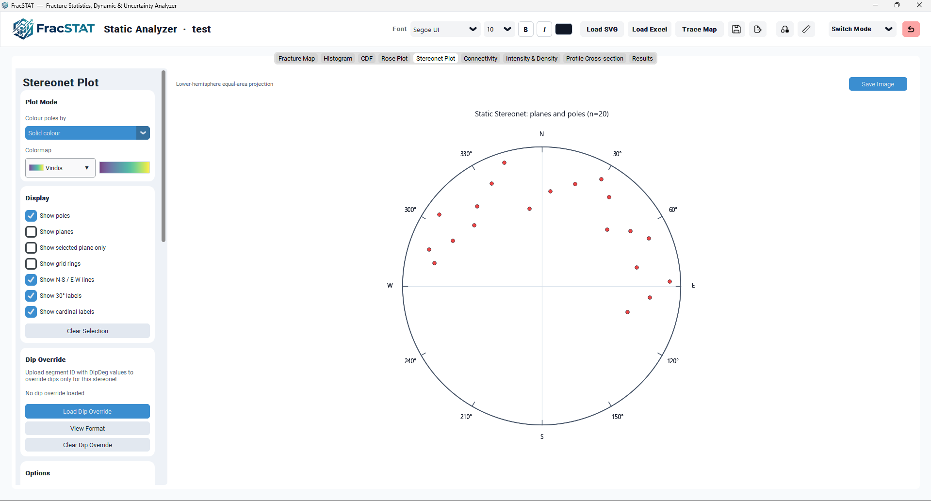
The Stereonet Plot tab uses the same two‑column layout as every other Static Analyzer tab: a scrollable control sidebar (fixed width, approximately 290 px) on the left, and a plot card occupying the remaining horizontal space on the right. The stereonet is drawn on a standard Cartesian Matplotlib Axes (not a polar Axes) sized 9 × 7 inches at 100 DPI — the equal‑area transformation is computed manually in Python and the resulting Cartesian (x, y) coordinates are plotted directly, giving the module full control over grid styling, labelling, and the great‑circle plane curves that would be awkward to render on a native polar projection.

Figure 1.1 — Full view of the Stereonet Plot tab, showing the left‑hand control sidebar (Plot Mode, Display, Dip Override, Options, Colours, Selected Pole, Statistics cards) and the right‑hand plot card containing the equal‑area stereonet and its colour bar.

1.1 Sidebar Card Structure

The sidebar is subdivided into seven bordered, rounded‑corner "cards", built top‑to‑bottom in the following order:

#	Card	Function
1	Plot Mode	Selects the attribute used to colour poles (strike, dip, length, or a solid colour) and the active Matplotlib colormap.
2	Display	Seven checkboxes controlling which graphical elements (poles, planes, grid, crosshairs, labels) are drawn, plus a Clear Selection button.
3	Dip Override	Upload, preview the format of, and clear a CSV/Excel file that substitutes per‑segment dip values for this diagram only.
4	Options	Custom plot title, colour‑bar position, pole marker shape, pole size, plane line width, and plane opacity.
5	Colours	Nine colour swatches and two numeric line‑width fields governing every drawable element's appearance.
6	Selected Pole	Read‑only text panel reporting the attributes of the currently picked fracture.
7	Statistics	Read‑only summary of plane count, circular mean strike, mean dip, and total mapped length.

1.2 Plot Card

The plot card contains a toolbar row (a caption reading "Lower‑hemisphere equal‑area projection" and a Save Image button), the Matplotlib canvas hosting the stereonet itself, and — depending on the selected colour‑bar position — an auxiliary colour‑bar axis fused into the same figure.

1.3 Reset Defaults

A single Reset Defaults button at the base of the sidebar restores every styling variable (colours, sizes, toggles, custom title) to its factory value and immediately redraws the diagram. It does not clear loaded fracture data, dip overrides, or the current pole selection.

2. Data Input

2.1 Source of Fracture Data

The Stereonet Plot tab does not load files itself. It reads directly from self.results, the shared pandas DataFrame populated by the Static Analyzer's map‑geometry engine whenever an SVG trace map or an Excel/CSV orientation table is loaded via the workspace header's Load SVG / Load Excel buttons, or whenever the profile scale, Y‑axis azimuth, or reverse‑Y setting is changed and geometry is recalculated. Because every Static Analyzer tab consumes the same results table, the stereonet, the fracture map, the rose diagram, the CDF, and the results table are always mutually consistent for a given dataset.

2.2 Required and Optional Columns

Column	Required	Description
StrikeDeg	Yes	Fracture strike measured from North, stored as a fully‑directed value in the 0–360° domain. Folded to 0–180° internally for orientation statistics where direction of dip is irrelevant, but the full 0–360° value is retained wherever dip direction matters.
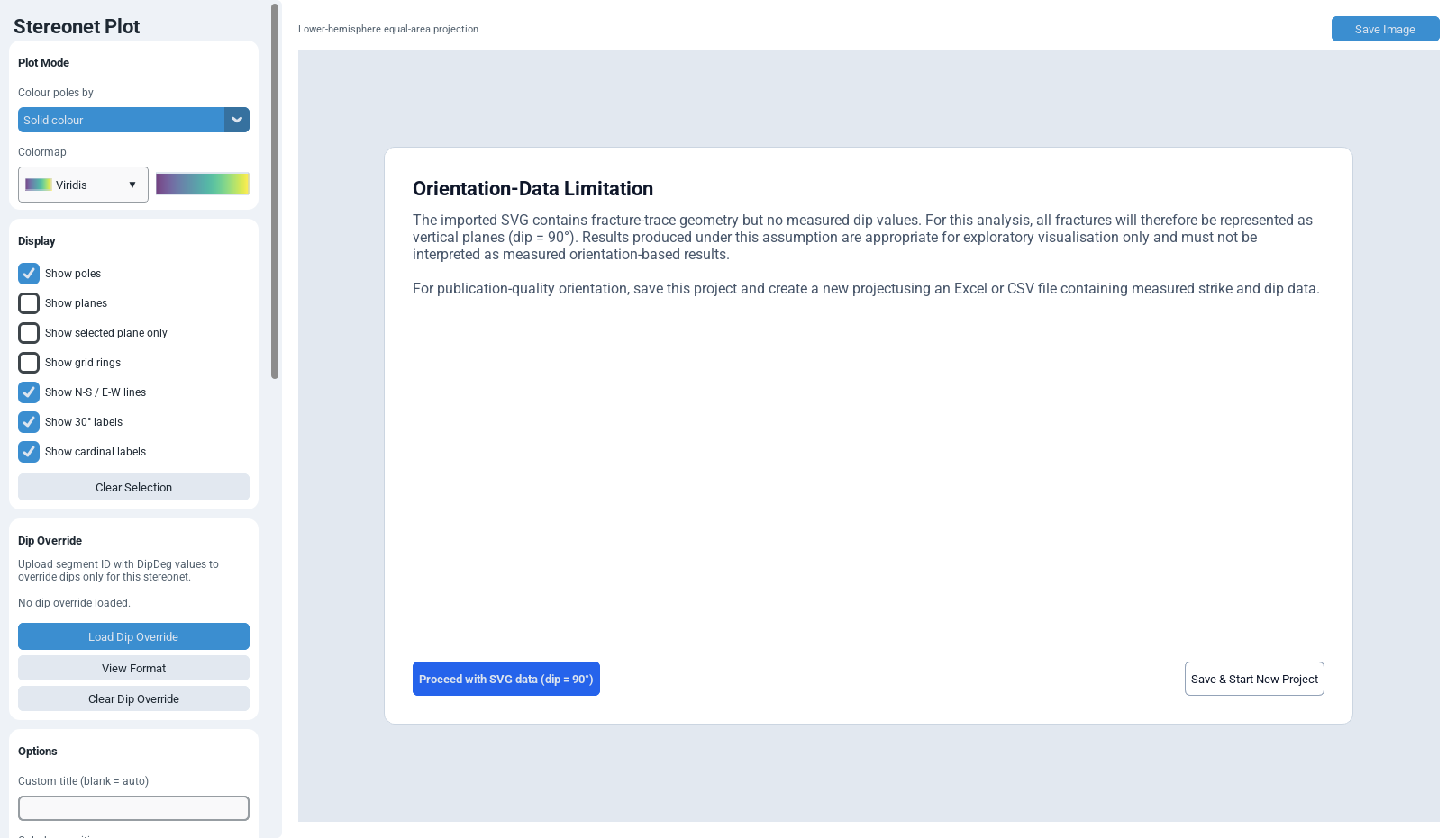
DipDeg	No (defaults to 90°)	Dip angle of the fracture plane, 0–90°. If absent, every segment is treated as a vertical fracture (90°) — the typical situation for a two‑dimensional SVG trace map with no independently measured dip.
DipDirection	No	Optional dip‑azimuth column present in some legacy Excel fracture‑plane files. When populated for a row, it overrides that row's strike via the right‑hand‑rule relationship strike = (DipDirection − 90°) mod 360°.
ID	No	Integer segment identifier used to (a) match rows against an uploaded Dip Override file and (b) drive the cross‑tab pole‑selection mechanism.
Length_m	No	Real‑world segment length in the project's active display unit; used only for the "Length colour" plot mode and the Total Length statistic.

2.3 Excel/CSV Orientation Formats Accepted Upstream

Although the Stereonet Plot tab itself is format‑agnostic (it only ever sees the already‑parsed results table), it is useful to record which upstream input formats can populate StrikeDeg/DipDeg: (1) raw segment/results tables carrying explicit X1, Y1, X2, Y2 endpoints and a pre‑computed StrikeDeg; (2) the legacy fracture‑plane format (ID, Strike, Dip, optional Trace, Dip Direction, Length, Aperture); (3) pole‑orientation tables (Trend, Plunge), automatically converted to strike/dip; and (4) focal‑mechanism tables (Lat, Lon, FP1/FP2 Strike/Dip/Slip), used primarily by the Dynamic Analyzer but also readable here. Regardless of the source format, the Stereonet Plot tab treats every row identically once StrikeDeg and DipDeg exist in the results table.

2.4 Row‑Level Validation

On every redraw the module performs the following validation sequence before any geometry is computed:

1. Strike values are read and wrapped into the 0–360° domain via a modulo operation, guaranteeing a well‑defined azimuth even if upstream data supplied negative or over‑range values.
2. If a DipDeg column exists, dip values are read directly; otherwise every row is assigned a default dip of 90°.
3. If a dip‑override dictionary is active (Section 3.3) and the results table carries an ID column, each row's dip is replaced with the corresponding override value wherever a finite override exists for that ID; rows without a matching override retain their original dip.
4. If a DipDirection column is present and finite for a given row, that row's strike is recomputed from the dip‑azimuth relationship described above, superseding the StrikeDeg value for that row only.
5. A combined finite‑value mask (numpy.isfinite) is applied to both strike and dip arrays; rows failing either test are dropped from the plotted set (and from the DataFrame passed onward to selection/statistics).
6. Surviving dip values are clipped to the physically valid 0–90° range with numpy.clip, protecting the projection mathematics from out‑of‑range inputs that could otherwise produce a negative argument to a square root.

If, after this pipeline, zero rows remain, the module displays an explanatory empty‑state message instead of attempting to draw an empty or degenerate diagram (see Section 7.5).

3. Settings and Controls, Card by Card

Unless stated otherwise, every control triggers an immediate redraw through _draw_static_stereonet, so changes are reflected on the canvas without a separate "apply" step.

3.1 Card 1 — Plot Mode

Control	Widget	Default	Options / Range	Effect
Colour poles by	Dropdown	Solid colour	Strike colour, Dip colour, Length colour, Solid colour	Selects which quantity is mapped to pole colour. See Section 4.5 for the exact value and normalisation used by each mode.
Colormap	Custom colour‑gradient dropdown with live 104×28 px swatch preview	Viridis	Any of the 23 named colour scales in the shared colour‑scale catalogue (Turbo, Jet, Parula, Hot, Bone, Viridis, Plasma, Inferno, Magma, Cividis, Coolwarm, HSV, Seismic, Spectral, Red‑Yellow‑Blue, Ocean, Terrain, Earth, Twilight, Copper, Yellow‑Green‑Blue, Grayscale, Blue‑White‑Red, Pink‑Yellow‑Green)	Determines the Matplotlib colormap object used whenever the active plot mode is not Solid colour. The Parula entry is a bespoke six‑stop MATLAB‑style colormap reproduced without an external dependency.

3.2 Card 2 — Display

Control	Widget	Default	Effect
Show poles	Checkbox	On	Toggles rendering of the pole‑point scatter layer. When off, the pick/selection scatter artist is set to None and picking is disabled.
Show planes	Checkbox	Off	Draws the full great‑circle trace for every fracture plane in the dataset, using the Plane Color/Plane width/Plane opacity settings. Suppressed automatically whenever "Show selected plane only" is active.
Show selected plane only	Checkbox	Off	When on and a pole is currently selected, only that fracture's great circle is drawn (in the Selected Pole colour, at 1.8× the configured plane width), instead of all planes.
Show grid rings	Checkbox	Off	Draws three dashed reference circles at 25%, 50%, and 75% of the net radius and twelve 30°‑spaced radial spokes from the centre to the boundary, all in the Grid Color.
Show N‑S / E‑W lines	Checkbox	On	Draws the two orthogonal diameters of the net (a simple crosshair) in the Grid Color at slightly higher opacity/width than the optional grid rings.
Show 30° labels	Checkbox	On	Draws tick marks and numeric/cardinal labels at every 30° increment around the boundary circle.
Show cardinal labels	Checkbox	On	When 30° labels are also on, substitutes N/E/S/W for the 0°/90°/180°/270° numeric labels. When 30° labels are off, this checkbox independently draws just the four cardinal letters at the circle's edge.
Clear Selection	Button	—	Deselects the currently picked fracture across the Stereonet, Fracture Map, and any other tab that shares selected_segment_id, and redraws all affected views.

3.3 Card 3 — Dip Override

Because most fracture data enters FracSTAT as a two‑dimensional SVG trace map, every segment is initially assigned a uniform default dip (typically 90°, i.e. vertical). The Dip Override mechanism allows a user to assign realistic, per‑segment dip values — for example, values digitised from field notes or a companion borehole‑image survey — without altering the source SVG or the shared results table used elsewhere in the application. The override is scoped to the Stereonet Plot tab only; it does not affect the Fracture Map, Rose Plot, or the Dynamic Analyzer's own independent dip‑override mechanism.

Control	Widget	Effect
Load Dip Override	Button + file dialog	Opens a file picker restricted to .csv, .xlsx, and .xls files. The selected file is parsed with pandas.read_excel or pandas.read_csv depending on extension.
View Format	Button with hover/click preview card	Displays a floating card illustrating the two required columns (ID, DipDeg) with three worked example rows, so the user can format a spreadsheet correctly before uploading.
Clear Dip Override	Button	Discards the in‑memory override dictionary, restores every segment to its original (or DipDirection‑derived) dip, and updates the status label to "No dip override loaded."

3.3.1 File Parsing and Column Matching

Column headers are matched case‑insensitively and are tolerant of internal spaces, hyphens, and underscores: the header text is lower‑cased and every non‑alphanumeric character is stripped before comparison. The identifier column is matched against id, segmentid, fractureid, or fracture; the dip column is matched against dipdeg, dipdig, dipdegree, dipdegrees, fracturedip, fracturedipdeg, wholerockdip, or dip. If either column cannot be located, the load is rejected with an explanatory error dialog.

3.3.2 Validation Rules

• Rows with a missing ID or DipDeg value are dropped via pandas.DataFrame.dropna before processing.
• Every surviving DipDeg value must lie within the closed interval [0°, 90°]; if any row violates this bound, the entire file is rejected with a descriptive error and no partial override is applied.
• The identifier column is cast to Python int and the dip column to float; the resulting {segment_id: dip_value} dictionary is stored as self.static_stereo_dip_overrides and is also written into the launcher's cross‑workspace shared_Analyzer dictionary so that a later switch to the Dynamic Analyzer or a project reload can, where applicable, see the same override set.
• The status label beneath the buttons is updated to read "Loaded dips for N IDs." on success.

3.4 Card 4 — Options

Control	Widget	Default	Effect
Custom title (blank = auto)	Text entry	(empty)	When non‑empty, replaces the automatically generated title ("Static Stereonet: planes and poles (n=...)") with the user‑supplied text.
Colorbar position	Dropdown	Bottom	Bottom, Top, Left, Right, or None. Controls the placement and orientation of the colour‑bar axis; ignored entirely when the active plot mode is Solid colour, since no colour bar is meaningful in that case.
Pole shape	Dropdown	Circle	Circle (o), Diamond (D), Square (s), Triangle Up (^), Star (*), Cross (X). Selects the Matplotlib marker style used for every plotted pole.
Pole size	Numeric entry (points², Matplotlib scatter units)	30	Controls the on‑screen area of each pole marker.
Plane width	Numeric entry (line width, points)	0.85	Line width used when drawing great‑circle plane traces.
Plane opacity	Numeric entry (0–1)	0.35	Alpha transparency applied to plane traces; automatically clamped to the [0, 1] interval.

3.5 Card 5 — Colours

Every colour swatch in this card opens the shared FracSTAT colour‑picker dialog (a 40‑swatch preset palette plus a live hex‑code entry with preview) and, when a new colour is confirmed, immediately triggers a redraw.

Control	Default	Element Affected
Outer BG	#FFFFFF	Colour of the Matplotlib Figure background, i.e. the area outside the plotted Axes.
Plot BG	#FFFFFF	Colour of the Axes background (the interior of the stereonet's bounding square, visible outside the circular net boundary).
Grid Color	#D9E2EC	Colour used for the optional 25/50/75% reference rings, the 30° radial spokes, and (when enabled) the N‑S/E‑W crosshair.
Boundary	#475569	Colour of the primary bounding circle and, when 30° labels are enabled, the associated tick marks.
Boundary width	1.2	Line width (points) of the bounding circle.
Pole Color	#EF4444	Fill colour of pole markers when the active plot mode is Solid colour.
Pole Border	#111827	Edge colour drawn around every pole marker regardless of plot mode.
Pole border width	0.45	Line width (points) of the pole marker edge.
Plane Color	#2563EB	Colour of great‑circle plane traces (Show planes).
Selected Pole	#00D4FF	Colour used for the highlight rings, the "P" marker, and (if enabled) the selected plane's great circle when a fracture is picked.

3.6 Card 6 — Selected Pole

A read‑only, left‑justified text label reporting five fields for the most recently picked fracture: ID, Plane strike (°), Plane dip (°), Pole trend (°), and Pole plunge (°). Before any selection is made, or after Clear Selection is pressed, the label reads "No pole selected." The pole trend and plunge reported here are the true orientation of the pole vector itself (trend = strike − 90°, mod 360°; plunge = 90° − dip), which is distinct from — and complementary to — the plane's own strike and dip.

3.7 Card 7 — Statistics

Statistic	Computation
Planes	Count of valid rows surviving the validation pipeline of Section 2.4 (n).
Mean Strike	Circular (axial) mean of all strikes folded to the 0–180° domain, computed by the doubling‑angle method described in Section 4.4; reported to one decimal place.
Mean Dip	Arithmetic (linear) mean of the dip array, via numpy.nanmean; reported to one decimal place. A linear mean is appropriate for dip because, unlike strike, dip is a bounded, non‑circular quantity.
Total Length	Sum of the Length_m column across all valid rows (0 if the column is absent), reported with the active display unit suffix (m, cm, mm, or km, per the Static Analyzer's profile‑unit selector).

3.8 Non‑Sidebar Controls

Control	Location	Effect
Save Image	Plot‑card toolbar	Exports the current figure as a 300 dpi PNG (or the project‑configured export DPI) to the project's FracSTAT_plot_exports folder, using the shared save_plot_image routine common to every Static Analyzer tab.
Pole picking (mouse click)	Directly on the canvas	Clicking within a marker's pick radius (6 px) selects that fracture; see Section 5.4.
Reset Defaults	Bottom of sidebar	Restores every styling variable listed in Sections 3.1–3.5 to its factory default (see Section 11.3) and redraws.

4. Mathematical Background

4.1 The Lower‑Hemisphere Equal‑Area (Schmidt) Projection

A stereonet is a two‑dimensional projection of the lower half of a reference sphere (the "projection hemisphere") used throughout structural geology to plot the orientation of lines and planes. FracSTAT implements the equal‑area (Schmidt, or Lambert azimuthal equal‑area) variant rather than the equal‑angle (Wulff) variant, because equal‑area projections preserve angular area — a critical property for any subsequent density‑contouring or population‑statistics work, since it guarantees that a uniformly random population of orientations produces a uniform point density on the diagram (Ragan, 2009; Allmendinger et al., 2012). The same convention is used by the established stereographic-projection packages in structural geology, so diagrams produced here are directly comparable with theirs (Cardozo and Allmendinger, 2013).

For a line with trend T (measured clockwise from North, 0–360°) and plunge P (measured downward from horizontal, 0–90°, positive), the module computes the projected Cartesian position (x, y) with the following transformation, implemented in the static method _static_stereo_line_point:

This is the standard Lambert azimuthal equal‑area formula expressed in colatitude form (Snyder, 1987). At P = 90° (a vertical line, plunging straight down), θ = 0° and r = 0, placing the point at the centre of the net, exactly as expected for a line piercing the lower hemisphere at its pole. At P = 0° (a horizontal line), θ = 90° and r = √2·sin(45°) = 1, placing the point exactly on the unit‑radius bounding circle.

4.2 From Plane Strike/Dip to Pole Position

Every fracture segment in the results table is characterised by a strike (the compass bearing of the horizontal line of intersection between the fracture plane and a horizontal reference plane) and a dip (the maximum angle of inclination of the plane, measured downward from horizontal, perpendicular to strike). The pole of a plane is the unit vector normal to that plane; plotting poles rather than the planes themselves is the conventional way to visualise large fracture populations, since a cluster of points is far easier to read than a cluster of overlapping great‑circle arcs (Priest, 1993).

The relationship between a plane's strike/dip and its pole's trend/plunge, using the right‑hand rule convention adopted throughout FracSTAT (dip direction = strike + 90°) (Allmendinger et al., 2012), is:

Substituting these into the colatitude form of Section 4.1 gives θ = 90° − pole plunge = dip, so that the pole radius can be computed directly from dip without an intermediate plunge calculation:

This is the exact computation performed for every row of the results table inside _draw_static_stereonet, applied as a fully vectorised NumPy operation across the entire (filtered) fracture population in a single pass rather than looping row by row.

4.3 Great‑Circle Trace of a Plane

When "Show planes" (or "Show selected plane only") is enabled, the module draws the complete great‑circle trace of each plane — the projected image of every point on the plane that intersects the reference sphere — rather than only its single pole point. The static method _static_stereo_plane_curve constructs this curve geometrically as follows, for a plane of strike S and dip D:

1. Two orthonormal in‑plane basis vectors are built in an (East, North, Up) coordinate frame: a strike vector s = (sin S, cos S, 0) lying along the horizontal strike line, and a down‑dip vector d = (sin(S+90°)·cos D, cos(S+90°)·cos D, −sin D) pointing down the dip direction into the plane.
2. A parameter t is swept across 140 equally spaced values from 0 to π radians, and for each value a unit vector on the plane is formed by v(t) = s·cos(t) + d·sin(t). Sweeping only 0 to π (rather than the full 0 to 2π) is sufficient because the lower‑hemisphere projection is symmetric: t and t+π map to antipodal points that, for a plane's great circle, coincide with the same lower‑hemisphere trace.
3. Each direction vector v(t) = (v_E, v_N, v_U) is converted to a plunge and trend: plunge = arcsin(−v_U), trend = atan2(v_E, v_N).
4. Every (trend, plunge) pair is projected with the same equal‑area formula as Section 4.1: radius = √2·sin((90° − plunge)/2), x = radius·sin(trend), y = radius·cos(trend).

The resulting 140‑point polyline, plotted with Matplotlib's standard line‑drawing routine, renders as the smooth, gently curved great‑circle arc familiar from printed stereonet overlays. Because the whole curve is generated with vectorised trigonometric NumPy calls, its cost is negligible even for a moderately sized fracture population.

4.4 Circular (Axial) Mean of Strike

Strike is an axial (180°‑periodic) rather than a directional (360°‑periodic) quantity: a fracture striking 010° is geologically identical to one striking 190°. A naive arithmetic mean of strike angles is therefore meaningless whenever a population straddles the 0°/180° wrap‑around boundary (for example, strikes of 179° and 1° should average to approximately 0°/180°, not 90°). FracSTAT resolves this with the standard doubling‑angle circular‑statistics technique (Mardia and Jupp, 2000, §2.3.2), implemented in _static_stereonet_axial_mean:

where θᵢ is each fracture's strike folded to the 0–180° domain, and wᵢ is a uniform‑weight contribution factor (the Statistics card currently applies uniform weighting rather than a length‑weighted option). Doubling every angle before applying the standard circular‑mean formula collapses the 180° periodicity into a 360° periodicity, allowing the ordinary vector‑sum trigonometric identity to be applied; halving the resulting angle and folding it back into 0–180° recovers the correct axial mean.

4.5 Colour Normalisation

Depending on the active Plot Mode, pole colours are mapped through a Matplotlib Normalize object with one of the following fixed or data‑driven ranges:

Plot Mode	Quantity Mapped	Normalisation Range
Dip colour	DipDeg	Fixed [0°, 90°] — the full physically valid dip range, regardless of the actual data spread, so that colour comparisons remain meaningful across different datasets and sessions.
Length colour	Length_m	Data‑driven [0, max(Length_m)] — rescaled to the current dataset's maximum observed length; degenerates gracefully to a minimum span of 1×10⁻⁹ if the maximum is zero or the column is missing.
Strike colour	StrikeDeg mod 180°	Fixed [0°, 180°] — the full axial strike domain.
Solid colour	(none)	No colour bar; every pole uses the single configured Pole Color.

5. Algorithms

5.1 Data Preparation Pipeline

Every invocation of the draw routine (_draw_static_stereonet) begins by re‑deriving the plottable strike/dip arrays from scratch rather than caching a previous computation, ensuring the diagram always reflects the current state of dip overrides, DipDirection substitutions, and the active selection. The pipeline is:

1. Read StrikeDeg and, if present, DipDeg from self.results; wrap strike into 0–360° via a modulo operation and default missing dip data to a constant array of 90°.
2. Apply the dip‑override dictionary, matched by integer ID, using numpy.where to substitute only the rows for which a finite override value exists, leaving all other rows untouched.
3. Apply any DipDirection‑derived strike override, again via numpy.where, only for rows where DipDirection is finite.
4. Build a combined boolean validity mask with numpy.isfinite on both strike and dip arrays; index both arrays and the results DataFrame with this mask to obtain the final plottable subset (df_valid).
5. Clip the surviving dip values into [0°, 90°] with numpy.clip as a final safety net against any residual out‑of‑range values.

5.2 Colour Resolution

Colour resolution is a two‑stage lazy lookup designed to avoid repeatedly importing the Dynamic Analyzer's colour‑scale catalogue module on every redraw. The user‑facing dropdown stores a human‑readable display name (e.g. "Viridis"); a companion callback (_on_cmap_change), fired whenever the dropdown selection changes, resolves that display name through the shared colour‑scale definition catalogue into (a) a genuine Matplotlib colormap identifier string and (b) — for the single special case of "Parula", which has no native Matplotlib equivalent — a bespoke LinearSegmentedColormap built from six manually specified hex‑colour control points. The resolved identifier is cached in self.static_stereo_cmap_resolved so that subsequent redraws (_static_stereo_cmap) can retrieve the ready‑made colormap object without re‑parsing the dropdown text or re‑touching the catalogue.

5.3 Pole Colour‑Value Selection

The helper _static_stereo_values(df, strikes, dips) is a small dispatcher that returns a (values, axis_label, Normalize) triple appropriate to the current Plot Mode, implementing the normalisation ranges tabulated in Section 4.5. When the plot mode is Dip colour, it returns the dip array directly. When it is Length colour and a Length_m column exists, it substitutes any non‑finite length with 0.0 (via numpy.where) before computing the data‑driven maximum, preventing a single corrupt or missing value from breaking the colour scale for the entire population. For every other case (including the default Strike colour fallback used whenever Length colour is selected but no length data exists) it returns the strike array folded into the 0–180° domain.

5.4 Selective Plane Rendering

The module draws great‑circle traces in one of three mutually exclusive states, resolved before the main pole scatter is built: (a) if "Show planes" is on and "Show selected plane only" is off, every valid fracture's great circle is drawn in a single loop using the shared Plane Color/width/opacity; (b) if "Show selected plane only" is on and a fracture is currently selected, only that fracture's great circle is drawn, in the Selected Pole colour at an emphasised (1.8×) line width and full 0.95 opacity, as part of the selection‑highlight sequence described below; (c) if neither toggle is active, no plane curves are drawn at all, leaving only the pole scatter.

5.5 Selection Highlight Rendering and Cross‑Tab Synchronisation

When self.selected_segment_id matches an ID present in the filtered dataset, the module renders a four‑layer highlight stack directly on top of the ordinary pole scatter, in ascending z‑order: (1) a large, thick, white‑edged open circle ("halo") of size max(180, pole_size×4.0); (2) a slightly smaller dark‑edged open circle of size max(125, pole_size×2.8); (3) a filled "P"‑shaped (plus/star) marker in the Selected Pole colour, sized max(62, pole_size×1.6); and (4) a text annotation reading "ID {n}" offset ten points to the upper right, rendered inside a rounded, semi‑opaque background box for legibility against any underlying grid or pole cluster. This layered halo approach guarantees the selected fracture remains visually unambiguous even in a dense, highly overlapping pole cloud.

Picking is implemented via Matplotlib's native artist‑picking API rather than a manual hit‑test: the pole scatter artist is created with picker=True and pickradius=6 (a six‑pixel tolerance radius around each rendered marker centre), giving a consistent, predictable click target in screen‑pixel space regardless of how many poles are compressed into the net. Clicking a pole fires Matplotlib's pick_event, handled by _on_static_stereonet_pick, which verifies the picked artist matches the current pick artist reference, reads the ID of the first matched index, and assigns it to self.selected_segment_id — the same shared attribute used by the Fracture Map tab and (for orientation‑only Excel data) the Results tab. Immediately afterward, if the Fracture Map's own draw method exists on the instance, it is invoked so the map's highlight ring updates in lockstep with the stereonet's, and finally the stereonet itself is redrawn. Clear Selection (_clear_static_stereonet_selection) performs the symmetric operation: it nulls the selection, clears the info panel, and triggers the same two‑tab redraw.

5.6 Stereonet Frame Construction

The frame — the fixed scaffold of circles, grid lines, and labels that gives the plot its stereonet appearance — is built by _format_static_stereonet and is invoked twice per redraw: once at the start of _draw_static_stereonet (to establish axis limits before any data is plotted) and once again at the end (so that frame elements such as the bounding circle are guaranteed to sit visually above the pole/plane layers, since Matplotlib's default z‑ordering follows draw order). The construction sequence is:

1. Fix the Axes aspect ratio to 1:1 and the view limits to [−1.15, 1.15] on both axes, then disable all default Matplotlib axis chrome (axis('off')).
2. Draw the unit‑radius bounding circle using 361 uniformly sampled angle steps.
3. If grid rings are enabled, draw three concentric dashed circles at fractional radii 0.25, 0.5, 0.75 and twelve 30°‑spaced spokes from the origin.
4. If the crosshair toggle is enabled, draw the two orthogonal N‑S and E‑W diameters.
5. Render either full 30°‑spaced tick/label sets (optionally cardinal‑letter‑substituted at the four principal directions) or, when the 30°‑labels toggle is off but the cardinal toggle remains on, just the four N/E/S/W letters positioned outside the circle.

5.7 Main Draw Routine — Complete Sequence

The complete draw sequence executed by _draw_static_stereonet, in order, is:

1. Guard clause: if the Matplotlib Axes has not yet been created (tab not yet built), return immediately.
2. Read all styling variables (colours, widths, sizes) from their CTk StringVar/BooleanVar containers, with defensive float() parsing wrapped in try/except so that a malformed numeric entry silently falls back to its documented default rather than raising an exception that would freeze the UI.
3. Clear the primary Axes and the colour‑bar Axes; hide the colour‑bar Axes by default (it is only re‑shown later if the active plot mode actually needs one).
4. Set the Figure and Axes background colours from the Outer BG / Plot BG swatches.
5. Call _format_static_stereonet once to establish the frame, boundary circle, and optional grid/crosshair/label elements.
6. Guard clause: if self.results is empty, missing, or lacks a StrikeDeg column, render the empty‑state message and return.
7. Execute the full data‑preparation pipeline of Section 5.1.
8. Guard clause: if zero rows survive validation, render an alternative empty‑state message ("No valid strike/dip data found") and return.
9. Resolve the active colormap via _static_stereo_cmap().
10. Branch on plot mode: for Solid colour, set a flat pole_colors value and skip the colour‑bar entirely; otherwise call _static_stereo_values to obtain per‑pole colour values, build a ScalarMappable for the colour bar, and colour each pole via cmap(norm(values)).
11. If plane rendering is requested (case (a) of Section 5.4), loop over every valid row and plot its great‑circle trace before the poles are drawn, so poles visually sit on top of the plane curves.
12. Compute pole trend, pole radius, and Cartesian (x, y) for the entire valid population in one vectorised block (Section 4.2).
13. If "Show poles" is enabled, draw the full pole scatter with picker=True and pickradius=6, storing the returned artist for the pick_event handler to recognise; otherwise set that artist reference to None, which also disables picking.
14. If a selection is active and its ID is present in the valid subset, execute the selection‑highlight and (optionally) selected‑plane‑only rendering described in Section 5.4/5.5, and populate the Selected Pole info panel.
15. Call _format_static_stereonet a second time, so frame elements are guaranteed to be layered above the data.
16. Configure the colour bar via _setup_static_stereo_colorbar (Section 7.4).
17. Set the plot title (custom or auto‑generated, embedding the live fracture count n).
18. Call _static_stereonet_update_stats to refresh the Statistics card.
19. Request a canvas redraw via draw_idle(), which defers the actual paint operation to Qt's next idle cycle for smoother responsiveness under rapid successive control changes.

The module additionally exposes a public refresh_static_stereonet() hook, called by the Static Analyzer's shared refresh_all_tabs sequencing routine whenever new geometry has been calculated (a new file load, a profile‑scale change, or a global font/appearance change), guaranteeing the stereonet stays synchronised with the rest of the workspace without the tab needing to poll for changes itself.

6. Statistical Methods

6.1 Summary of Implemented Statistics

Statistic	Type	Formula / Method	Interpretation
Planes (n)	Count	Row count of the validated subset	Effective sample size underlying every other statistic and the colour normalisation.
Mean Strike	Circular (axial) mean, 180°‑periodic	Doubling‑angle vector‑resultant method, Section 4.4	The population's dominant fracture‑strike orientation; robust to the 0°/180° wrap‑around ambiguity inherent to axial (non‑directional) strike data.
Mean Dip	Linear (arithmetic) mean	numpy.nanmean(dip array)	Average steepness of the fracture population; a linear mean is statistically appropriate because dip is bounded (0–90°) and non‑circular.
Total Length	Sum	Σ Length_m across valid rows	Aggregate mapped fracture length in the dataset's active display unit; contextualises the population size in physical (as opposed to purely count‑based) terms.

6.2 Why Circular Statistics Are Required for Strike

Ordinary (linear) descriptive statistics assume that the underlying measurement scale is unbounded and that a small numerical difference always corresponds to a small physical difference. Compass bearings and, more specifically, axial strike measurements violate this assumption at the wrap‑around boundary: 179° and 1° are numerically 178° apart but geologically almost coincident (both describe an approximately N–S striking fracture set, once the 180° axial periodicity is accounted for). Using an arithmetic mean on such data can produce a wildly misleading result — in the worst case, a mean strike diametrically opposed to the true dominant orientation. The doubling‑angle technique used here (Section 4.4) is the standard remedy from directional statistics (Fisher, 1993; Mardia and Jupp, 2000) and is used consistently across FracSTAT's Rose Plot, Static Stereonet, and Results‑tab summary statistics.

6.3 Statistics as a Quality‑Control Tool

Because the Statistics card recomputes on every redraw, it functions as a live sanity check for the Dip Override workflow: after loading an override file, a user can immediately verify that the Mean Dip value has shifted in the expected direction and that the Planes count still matches the expected fracture population size, catching upload errors (mismatched IDs, wrong‑unit dip values, or a partially failed match) before the data is carried forward into any downstream stress analysis in the Dynamic Analyzer.

7. Visualization & Figure Components

7.1 Figure and Canvas Architecture

The stereonet is rendered on a single Matplotlib Figure (default size 9×7 inches at 100 dpi) embedded in the Qt plot card via FigureCanvasTkAgg. A secondary Axes, added into the same Figure at a fixed rectangle via add_axes, hosts the colour bar and is toggled visible/invisible depending on plot mode and user preference, avoiding the overhead of destroying and rebuilding Axes objects on every redraw.

7.2 Visual Element Inventory

Element	Always Drawn?	Controlled By
Bounding circle	Yes	Boundary colour / Boundary width
Grid reference rings (25/50/75%) + spokes	No	Show grid rings + Grid Color
N‑S / E‑W crosshair	No	Show N‑S / E‑W lines + Grid Color
30° tick marks + numeric/cardinal labels	No	Show 30° labels (+ Show cardinal labels for letter substitution)
Cardinal‑only labels (no ticks)	No	Show cardinal labels when 30° labels is off
Great‑circle plane traces (all planes)	No	Show planes (and Show selected plane only = off)
Great‑circle plane trace (selected only)	No	Show selected plane only, requires an active selection
Pole scatter	No (but default on)	Show poles
Selection halo (4‑layer highlight + ID label)	No	Requires an active, currently‑valid selection
Colour bar	No	Colorbar position ≠ None and plot mode ≠ Solid colour
Plot title	Yes	Custom title override or auto‑generated "Static Stereonet: planes and poles (n=...)"

7.3 Colour Bar Rendering

When active, the colour bar is built from the same ScalarMappable object used to colour the poles, guaranteeing an exact, artifact‑free correspondence between marker colour and the numeric scale. The colour‑bar label text is drawn using the module's muted text colour and automatically reflects the active plot mode ("Strike (°)", "Dip (°)", or "Length (<unit>)", where <unit> is the Static Analyzer's currently selected display unit — m, cm, mm, or km).

7.4 Colour‑Bar Layout Management

_setup_static_stereo_colorbar dynamically repositions both the colour‑bar Axes and the primary stereonet Axes as a matched pair, since adding a colour bar necessarily shrinks the space available to the stereonet itself. Four fixed layout presets are hard‑coded, one per colour‑bar position choice:

Position	Colour‑bar rectangle (figure fraction)	Orientation	Stereonet Axes rectangle
Bottom	[0.16, 0.085, 0.68, 0.032]	Horizontal	[0.10, 0.18, 0.80, 0.74]
Top	[0.16, 0.91, 0.68, 0.032]	Horizontal	[0.10, 0.06, 0.80, 0.78]
Left	[0.06, 0.17, 0.03, 0.66]	Vertical	[0.17, 0.08, 0.74, 0.84]
Right	[0.92, 0.17, 0.03, 0.66]	Vertical	[0.08, 0.08, 0.74, 0.84]

When the position is set to None, or the active plot mode is Solid colour (which has no meaningful colour scale to display), the colour‑bar Axes is hidden entirely and the stereonet Axes is expanded to a single centred [0.10, 0.08, 0.80, 0.84] rectangle, maximising the usable plotting area.

7.5 Title Construction and Empty/Error States

If the Custom Title field is left blank, the module auto‑generates a title of the form "Static Stereonet: planes and poles (n={count})", where {count} is the live number of valid, plotted fracture poles — giving the reader an immediate population‑size context without needing to consult the separate Statistics card.

7.6 Image Export

The Save Image toolbar button calls the Static Analyzer's shared save_plot_image routine, which writes the current Figure to a timestamped PNG file inside a per‑project FracSTAT_plot_exports subfolder, using the project‑configured export DPI (default 300, adjustable in the application‑wide Settings page). Because the export routine saves the live Matplotlib Figure object directly, the exported image is pixel‑for‑pixel identical to the on‑screen render, including every custom colour, label, and selection highlight active at the moment of export.

8. Step‑by‑Step Example Workflows

8.1 Example 1 — Basic Orientation Review of an SVG Trace Map

1. Load a digitised fracture trace map via the workspace header's Load SVG button. Every segment initially receives a default dip of 90°.
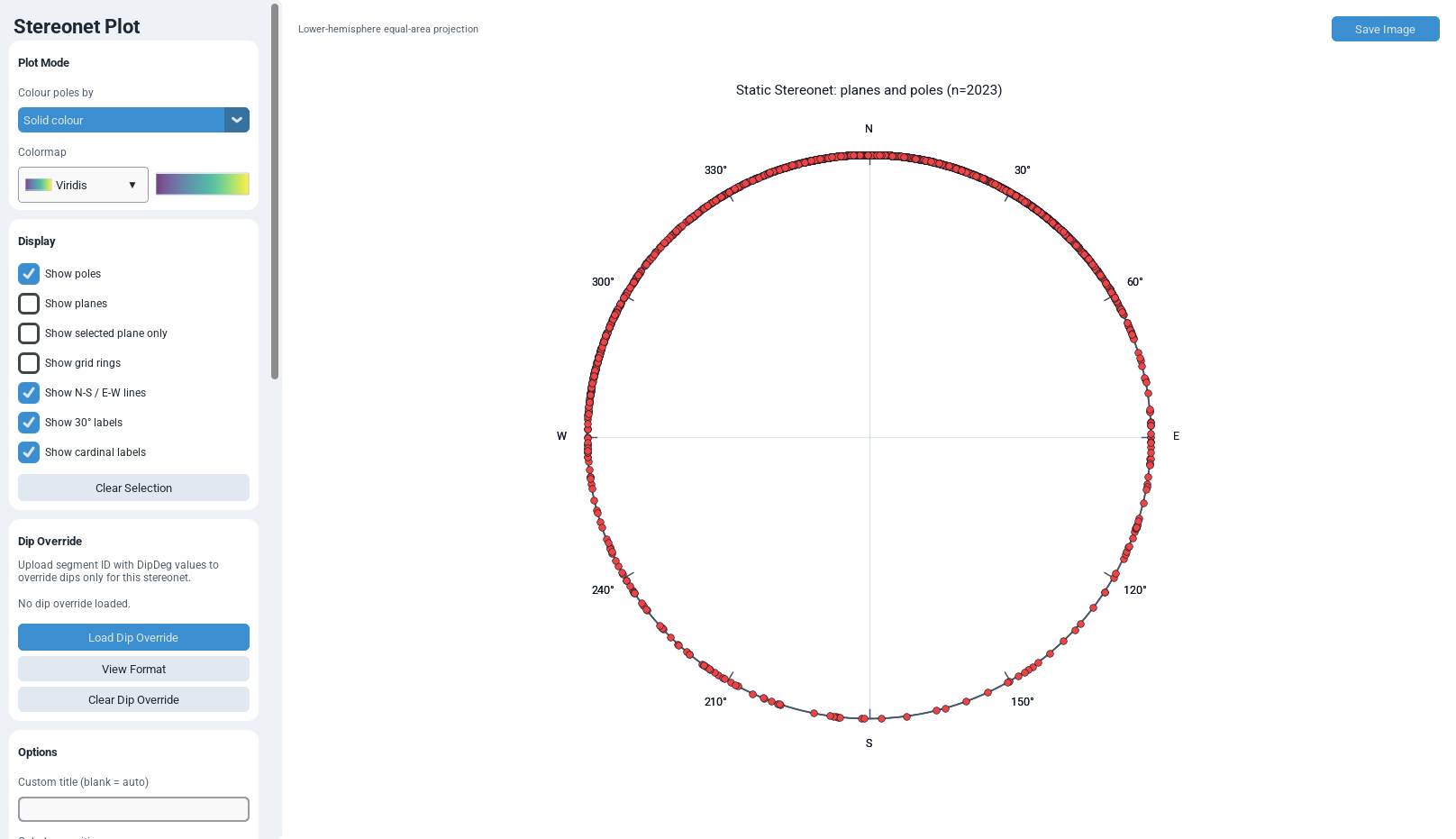
2. Open the Stereonet Plot tab. With Plot Mode left at its default Solid colour, every pole appears at the outer boundary circle (since dip = 90° corresponds to pole radius = 1), forming a ring pattern that directly visualises the strike distribution around the compass.
3. Switch Plot Mode to Strike colour and enable Show grid rings and Show 30° labels to add angular reference context.
4. Read the Statistics card: the Mean Strike value reports the population's dominant azimuth using the axial circular mean, and the Planes count confirms the number of segments successfully digitised.

8.2 Example 2 — Incorporating Field‑Measured Dips

1. Prepare a two‑column spreadsheet with headers ID and DipDeg, where ID values match the segment identifiers shown in the Static Analyzer's Table/Results tab, and DipDeg holds field‑measured dip angles in the 0–90° range.
2. In the Dip Override card, click View Format to confirm the expected layout, then click Load Dip Override and select the prepared file.
3. Observe that the pole ring on the stereonet collapses inward toward the centre for every overridden segment, now correctly reflecting non‑vertical dip, while segments without a matching override remain on the outer boundary.
4. Switch Plot Mode to Dip colour to visually audit which segments received an override (moved inward, showing a graded colour) versus which retained the 90° default (fixed at the boundary colour extreme).

8.3 Example 3 — Identifying Conjugate Fracture Sets

1. With a fully dip‑populated dataset loaded, enable Show planes to overlay every great‑circle trace.
2. Visually identify two angularly separated pole clusters; enable Show selected plane only and click a representative pole from each cluster in turn (the module keeps only the most recently picked selection, so compare one set at a time) to isolate and inspect each set's individual great circle against the full population.
3. Record the two clusters' mean orientations (readable from the Selected Pole panel for a representative fracture in each, or by filtering the source data and re‑loading a subset) and compute their angular separation to assess whether the pattern is consistent with a conjugate shear‑fracture pair.

8.4 Example 4 — Publication‑Quality Figure Preparation

1. Set a Custom title describing the dataset (for example, "Outcrop A — Joint Set Orientation, n = 248").
2. In the Colours card, select a colour palette consistent with the target publication's style guide (for example, switching Outer BG and Plot BG to white, and choosing a colour‑blind‑friendly colormap such as Viridis or Cividis for Length colour mode).
3. Set Colorbar position to Right for a compact, journal‑column‑friendly layout, and adjust Pole size and Boundary width for the target print resolution.
4. Click Save Image to export a high‑resolution PNG at the project's configured export DPI directly into the project's plot‑exports folder.

9. Geological Interpretation

9.1 Reading Pole Clusters

A tight cluster of poles indicates a single, well‑defined fracture set with consistent orientation — the geological signature of a systematic joint set formed under a single, spatially homogeneous stress or strain event. Multiple, angularly separated clusters typically indicate two or more distinct fracture sets, which may represent conjugate shear fractures (commonly separated by roughly 60–90° depending on the internal friction angle of the rock (Priest, 1993)), successive tectonic events with rotated principal stress axes, or a combination of systematic and non‑systematic (cross) joints. Because no clustering statistic is computed (Section 6.2), how tight a "tight" cluster is remains a visual judgement on this diagram; density contouring (Vollmer, 1995; Robin and Jowett, 1986) and eigenvalue fabric analysis (Woodcock, 1977) are the standard quantitative tools, and are not implemented here.

9.2 Girdle (Great‑Circle) Distributions

When poles are dispersed along a great‑circle arc rather than clustered at a point, the population is described as a girdle distribution. Geologically, a girdle commonly indicates that the fracture planes share a common axis of rotation or intersection — for example, fractures related to folding about a single fold axis, where the pole girdle's own great‑circle axis (its π‑pole) closely approximates the plunge and trend of the fold hinge (Ragan, 2009). The Show planes toggle, by drawing the actual great‑circle traces rather than only their poles, allows a user to visually confirm whether a suspected girdle arrangement of poles is indeed produced by planes sharing a common intersection line. Distinguishing a cluster from a girdle quantitatively requires the eigenvalues of the orientation tensor (Woodcock, 1977), which this tab does not compute.

9.3 Interpreting Colour‑Coded Attributes

• Strike colour (0–180°, cyclic‑appearing but linearly mapped) highlights orientation domains within a single diagram — useful for visually separating conjugate or cross‑cutting sets without needing a second plot.
• Dip colour (fixed 0–90° scale) is particularly informative for datasets combining vertical, SVG‑derived trace‑map fractures (typically defaulted to 90°) with dip‑override or directly measured fracture‑plane data, letting a user instantly distinguish which poles carry genuinely measured dip information versus assumed‑vertical defaults, since the latter will cluster tightly at the deep‑red or deep‑blue end of the fixed scale depending on the chosen colormap.
• Length colour reveals whether the longest, most laterally persistent fractures in the network share a common orientation with the shorter, more numerous population — a pattern often associated with a hierarchy of fracture generations (e.g. long master joints versus short cross joints).

9.4 Relationship to the Dynamic Analyzer

The purely geometric orientation fabric characterised here is the natural precursor to the Dynamic Analyzer's stress‑based slip‑tendency and Mohr‑Coulomb failure analysis: a fracture set identified as a tight, well‑defined cluster on this stereonet is a strong candidate for a mechanically significant, potentially reactivatable set once a stress tensor is applied (Morris et al., 1996; Zoback, 2007), whereas a poorly clustered or highly scattered population may indicate either genuine geological complexity (multiple superposed events) or a data‑quality issue (digitisation noise, an inappropriate default dip assumption) that should be resolved — for example via the Dip Override mechanism — before committing to a quantitative stress analysis.

9.5 Caution Regarding Default (Assumed) Dips

10. Performance Optimization

10.1 Vectorised NumPy Computation

Every geometric transformation described in Section 4 — strike wrapping, dip‑override substitution, pole trend/radius computation, and coordinate projection — is expressed as array‑level NumPy operations (modulo, where, clip, sin, cos, sqrt) applied to the entire fracture population simultaneously, rather than iterating row by row in pure Python. For typical FracSTAT datasets (tens to a few thousand fracture segments), this reduces the per‑redraw geometric computation to a negligible fraction of the overall render time, which is instead dominated by Matplotlib's own artist construction and canvas paint operations.

10.2 Great‑Circle Curve Cost Management

The great‑circle plane‑trace algorithm (Section 4.3) samples 140 points per plane, chosen as a balance between visual smoothness (no perceptible faceting on a typical screen or print render) and per‑plane computational and memory cost. Because plane rendering is opt‑in (Show planes defaults to off) and is itself vectorisable per plane, enabling it for populations of a few hundred fractures remains responsive; very large populations (several thousand fractures with planes enabled simultaneously) will show a proportional increase in draw time, and users working with such datasets are advised to use Show selected plane only, or to filter/subset the input data, rather than rendering every great circle at once.

10.3 Deferred Canvas Painting

The module calls the Matplotlib canvas's draw_idle() method rather than the blocking draw() at the end of every redraw. draw_idle() schedules the actual paint operation on Qt's event‑loop idle queue instead of forcing it synchronously, which allows several rapid, successive control changes (for example, quickly typing into a numeric entry field or dragging a colour picker) to coalesce into fewer physical repaints, improving perceived UI responsiveness without any explicit debounce logic in this module.

10.4 Colormap Resolution Caching

As described in Section 5.2, the resolved Matplotlib colormap identifier is cached in self.static_stereo_cmap_resolved after the dropdown's on‑change callback fires, so the hot draw path (_static_stereo_cmap) never needs to re‑parse the display name or re‑touch the shared colour‑scale catalogue on every redraw — it performs, at most, a single dictionary‑free conditional check and a call to matplotlib.cm.get_cmap.

10.5 Colour‑Bar Axis Reuse and I/O

Rather than creating and destroying a Matplotlib Axes object every time the colour bar is shown or hidden (an operation with non‑trivial overhead, since Axes creation touches the Figure's internal layout engine), the module creates the colour‑bar Axes exactly once, at tab‑construction time, and thereafter only toggles its visibility and repositions its bounding rectangle — consistent with the same pattern used across every other Static Analyzer plotting tab. The Stereonet Plot tab also performs no file or network I/O during normal redraw operation; the only I/O paths are the explicit, user‑initiated Load Dip Override file dialog and the Save Image export, both one‑shot operations outside the interactive redraw loop.

11. Advanced Features

11.1 Pole Marker Shape Library

Six marker shapes are exposed, mapped internally to Matplotlib single‑character/style codes:

Display Name	Matplotlib Marker Code	Typical Use
Circle	o	Default; neutral, high point‑density readability.
Diamond	D	Distinguishing a second fracture set on a comparative figure.
Square	s	Emphasis or grid‑aligned aesthetics for publication figures.
Triangle Up	^	Convention borrowed from many structural‑geology textbooks for a secondary population.
Star	*	High‑visibility marker for small, sparse populations.
Cross	X	Overlay marker style that remains legible atop dense clusters or a background image.

11.2 Dip‑Direction‑Aware Strike Correction

Certain upstream Excel fracture‑plane files record a plane's orientation via dip azimuth ("Dip Direction") rather than strike. Rather than requiring the user to pre‑convert this column, the Stereonet Plot tab applies the standard right‑hand‑rule inversion strike = (Dip Direction − 90°) mod 360° on a per‑row basis, silently overriding StrikeDeg only for the rows where a finite Dip Direction value is present. This allows a single results table to mix rows originating from strike‑based and dip‑direction‑based source files without any manual pre‑processing.

11.3 Reset Defaults

The reset routine (_static_stereonet_reset_defaults) writes the factory value into every corresponding StringVar/BooleanVar in a single pass — Plot mode to Solid colour, Colorbar position to Bottom, all colour swatches to their documented defaults, Pole shape to Circle and Pole size to 30, Plane width/opacity to 0.85/0.35, Show poles on with planes and selected‑plane off, grid rings off with crosshair/30°‑labels/cardinal‑labels on, and the Custom title cleared — then performs one redraw.

11.4 Shared Colour‑Scale Ecosystem

The colormap dropdown and its live‑swatch preview are implemented via the same CustomColorDropdown widget and colour‑scale catalogue used throughout FracSTAT (Dynamic Analyzer's Map/Rose/Mohr/Stereonet tabs, and the Static Analyzer's own Fracture Map, Intensity & Density, and Rose Plot tabs). This guarantees that a colour scale chosen here has visually identical appearance and semantics wherever else it is used in the application, and that any future addition to the shared catalogue automatically becomes available in this tab's dropdown without any change to this module.

11.5 Cross‑Workspace Dip Override State

Although the Dip Override loaded through this tab is scoped to the Static Analyzer's Stereonet Plot display, the resulting dictionary is also written into the launcher's shared shared_Analyzer['dip_overrides'] state slot. This is the same slot the Dynamic Analyzer's own, independently maintained dip‑override mechanism reads from when hydrating a freshly opened or mode‑switched workspace, meaning a dip override uploaded here can, depending on the exact sequence of workspace switches, become visible as a starting point in the Dynamic Analyzer as well — a convenience for users moving directly from geometric review to stress analysis, though it should not be relied upon as the primary path for setting Dynamic Analyzer dip overrides, which has its own dedicated upload control.

12. Limitations

Limitation	Description
Fixed default vertical dip	Dip values for fractures digitised purely from a two‑dimensional SVG trace map default to a fixed 90° (vertical) unless explicitly supplied via a DipDirection column in the source data or a Dip Override upload; the module cannot infer true three‑dimensional dip from plan‑view geometry alone. See Section 9.5.
No density contouring	Poles are plotted as discrete markers only. No contoured density estimate is computed, so overlapping markers obscure the true concentration in dense clusters and the visual impression depends on marker size. Standard contouring methods are those of Vollmer (1995) and Robin and Jowett (1986).
No fabric-shape or eigenvalue analysis	Cluster versus girdle versus random fabric is not quantified. The eigenvalues of the orientation tensor and the associated shape parameters (Woodcock, 1977) are not computed, so the interpretations in Section 9 rest on visual inspection.
No concentration or confidence statistics	No Fisher concentration parameter, confidence cone about a mean orientation, or test against a uniform distribution is reported (Fisher et al., 1987). Mean Strike and Mean Dip are point values only, and are computed independently of one another rather than as a true mean vector (Section 4.4).
No automatic set separation	Fracture sets are not clustered or classified automatically; assigning poles to sets is left to the user's judgement, and every statistic on the Statistics card is computed over the whole population rather than per set. For a bimodal population the reported means therefore describe neither set.
No orientation-bias correction	Poles are plotted as sampled. The Terzaghi weighting for orientation bias against fractures sub-parallel to the exposure or scanline (Terzaghi, 1965) is not applied, so apparent cluster strength partly reflects the sampling geometry.
Great-circle traces are discretised	Each plane's great circle is drawn from 140 sampled points, which is visually smooth at normal figure sizes but is an approximation; the curve is not analytically exact under extreme zoom or export scaling.

13. References

Sources are listed alphabetically within each group. In-text citations throughout this page link to the corresponding entry below.

13.1 Projection and Orientation Analysis

• Allmendinger, R. W., Cardozo, N., & Fisher, D. M. (2012). Structural Geology Algorithms: Vectors and Tensors. Cambridge University Press. https://doi.org/10.1017/CBO9780511920202
• Cardozo, N., & Allmendinger, R. W. (2013). Spherical projections with OSXStereonet. Computers & Geosciences, 51, 193–205. https://doi.org/10.1016/j.cageo.2012.07.021
• Fisher, N. I., Lewis, T., & Embleton, B. J. J. (1987). Statistical Analysis of Spherical Data. Cambridge University Press. https://doi.org/10.1017/CBO9780511623059
• Fisher, N. I. (1993). Statistical Analysis of Circular Data. Cambridge University Press. https://doi.org/10.1017/CBO9780511564345
• Mardia, K. V., & Jupp, P. E. (2000). Directional Statistics. John Wiley & Sons. https://doi.org/10.1002/9780470316979
• Ragan, D. M. (2009). Structural Geology: An Introduction to Geometrical Techniques (4th ed.). Cambridge University Press. https://doi.org/10.1017/CBO9780511816109
• Robin, P.-Y. F., & Jowett, E. C. (1986). Computerized density contouring and statistical evaluation of orientation data using counting circles and continuous weighting functions. Tectonophysics, 121(2–4), 207–223. https://doi.org/10.1016/0040-1951(86)90044-2
• Snyder, J. P. (1987). Map Projections — A Working Manual. U.S. Geological Survey Professional Paper 1395. https://doi.org/10.3133/pp1395
• Vollmer, F. W. (1995). C program for automatic contouring of spherical orientation data using a modified Kamb method. Computers & Geosciences, 21(1), 31–49. https://doi.org/10.1016/0098-3004(94)00058-3
• Woodcock, N. H. (1977). Specification of fabric shapes using an eigenvalue method. Geological Society of America Bulletin, 88(9), 1231–1236. https://doi.org/10.1130/0016-7606(1977)88<1231:SOFSUA>2.0.CO;2

13.2 Rock Engineering and Geomechanics

• Morris, A., Ferrill, D. A., & Henderson, D. B. (1996). Slip-tendency analysis and fault reactivation. Geology, 24(3), 275–278. https://doi.org/10.1130/0091-7613(1996)024<0275:STAAFR>2.3.CO;2
• Priest, S. D. (1993). Discontinuity Analysis for Rock Engineering. Chapman & Hall, London. https://doi.org/10.1007/978-94-011-1498-1
• Terzaghi, R. D. (1965). Sources of error in joint surveys. Géotechnique, 15(3), 287–304. https://doi.org/10.1680/geot.1965.15.3.287
• Zoback, M. D. (2007). Reservoir Geomechanics. Cambridge University Press. https://doi.org/10.1017/CBO9780511586477

13.3 Software

• Harris, C. R., Millman, K. J., van der Walt, S. J., Gommers, R., Virtanen, P., Cournapeau, D., … Oliphant, T. E. (2020). Array programming with NumPy. Nature, 585(7825), 357–362. https://doi.org/10.1038/s41586-020-2649-2
• Hunter, J. D. (2007). Matplotlib: A 2D graphics environment. Computing in Science & Engineering, 9(3), 90–95. https://doi.org/10.1109/MCSE.2007.55
• McKinney, W. (2010). Data structures for statistical computing in Python. Proceedings of the 9th Python in Science Conference, 56–61. https://doi.org/10.25080/Majora-92bf1922-00a