Static Intensity Tab

Located at static_analyzer/tabs/static_intensity_tab.py, the Intensity & Density tab (implemented as the mixin class TraceIntensityTab) is one of nine analytical workspaces within the FracSTAT Static Analyzer module. It implements a circular scanline sampling procedure — commonly attributed to Mauldon and co‑workers (Mauldon, 1998; Mauldon et al., 2001) — for the unbiased estimation of two fundamental fracture‑network descriptors used throughout structural geology, reservoir characterization, and rock‑mass engineering: P21 (areal fracture intensity — cumulative trace length per unit sampling area, units [length]/[length]² = [length]⁻¹) and P20 (areal fracture density — number of fracture traces per unit sampling area, units [length]⁻², in the P_ij notation of Dershowitz & Herda, 1992). P20 counts whole traces, never the straight segments a polyline trace happens to be digitised into: a single trace drawn with fifty vertices is one fracture, not fifty. Locally, the circular‑window estimator reaches the same quantity by counting trace tips inside the window, two tips per fully enclosed trace.

Unlike simple line‑scanline or box‑counting methods, the circular scanline technique is orientation‑independent: because a circle presents the same sampling window regardless of azimuth, P21 and P20 estimates computed from circular windows are not biased by preferential fracture orientation relative to the sampling geometry. This makes the method particularly well suited to anisotropic fracture networks, where a single straight scanline could over‑ or under‑sample fractures aligned sub‑parallel to it.

Within the broader FracSTAT workflow, this tab consumes the same segment‑level geometry (X1, Y1, X2, Y2, Length_m) produced by the Fracture Map tab's geometry engine, and therefore requires that a project already contain fracture trace data with real spatial coordinates — either digitized from an SVG trace map or imported from a spatially‑referenced Excel/CSV file. It complements the Connectivity tab (topological I‑Y‑X node analysis) and the Histogram/CDF tabs (length‑distribution statistics) by adding a spatially explicit measure of how fracture intensity varies across the mapped domain, rather than summarising the network as a single global statistic.

The tab produces both a spatially gridded (heatmap or kriged contour) representation of local P21/P20 and single‑value global P21/P20 statistics computed over the entire mapped area, giving the user both a map‑view understanding of intensity heterogeneity and a scalar summary suitable for reporting or comparison between datasets.

1. Purpose and Scope

The Intensity & Density tab exists to answer a question the Histogram, CDF, and Rose tabs cannot: not just how long or how oriented the fractures are, but how much fracturing exists per unit area, and how that quantity varies spatially across the mapped domain. The circular‑scanline (Mauldon) method was chosen specifically because it removes the directional sampling bias inherent in straight‑line scanlines, making the resulting P21/P20 estimates directly comparable between outcrops with different dominant fracture trends.

2. Interface Overview

The tab is built by the _build_trace_intensity_tab() method and follows the two‑column layout used throughout FracSTAT's Static Analyzer: a scrollable control sidebar on the left (approximately 280 px wide) and a plot canvas occupying the remaining space on the right. The sidebar is organised into five stacked cards, and the plot area contains a single Matplotlib figure embedded via FigureCanvasTkAgg, together with a compact toolbar.

Figure 2.1 — Full view of the Intensity & Density tab, showing the five sidebar cards (Settings, Plot Options, Map Elements, Background Image, Global Results) on the left and the rendered heatmap/contour plot on the right.

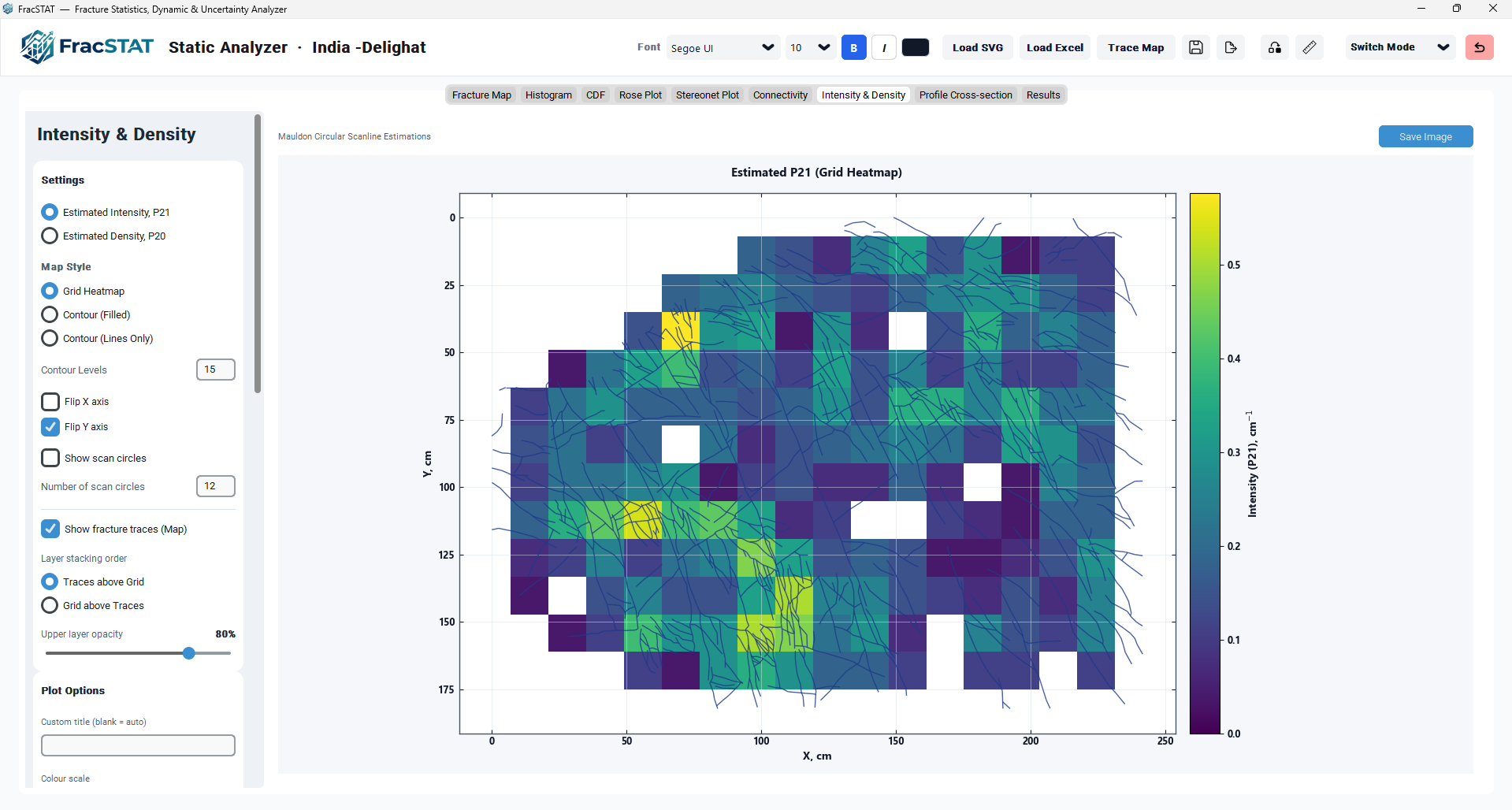
2.1 Sidebar Cards

Card	Purpose
Settings	Selects the statistic (P21/P20), the map rendering style (Heatmap/Contour), contour level count, axis flipping, scan‑circle overlay, circle count, and the trace/grid layering and opacity controls.
Plot Options	Custom plot title, colour‑scale (colormap) selector with a live gradient preview swatch, and colour‑bar position.
Map Elements	Colour pickers and toggle for outer/plot background, grid, trace colour, contour line colour, border colour/width, contour line width, and the show‑grid‑lines checkbox.
Background Image	Enables and configures an optional calibrated real‑world photograph drawn behind the intensity/density map, with an opacity slider.
Global Results	Read‑only statistics panel reporting the scan grid layout, total scan‑circle count, and the two headline global statistics: Global Intensity (P21) and Global Density (P20).

2.2 Plot Toolbar

A single‑row toolbar sits above the plot canvas. It displays a static caption, "Mauldon Circular Scanline Estimations", identifying the underlying method, and a Save Image button that calls the shared save_plot_image() routine (inherited from StaticAnalyzerApp) to export the current figure as a high‑resolution PNG into the project's FracSTAT_plot_exports folder, honouring the DPI configured on the Settings page.

2.3 Plot Canvas

The canvas is a single Matplotlib Axes (self.p21_ax) hosted inside a Figure (self.p21_fig) at 9×6 inches / 100 DPI. Depending on the selected style, the axes displays a pcolormesh heatmap, a filled/line contour plot (optionally kriged), the fracture trace network as a LineCollection, scan‑circle outlines, an optional scale bar in the lower‑right corner, and — if enabled — a background photograph. A colour bar is attached via fig.colorbar(..., location=...), but its position is then explicitly overridden by a custom alignment routine, _align_colorbar_to_plot(), rather than being left at Matplotlib's default constrained‑layout slot — see the note below.

3. Data Input Requirements

The Intensity & Density tab reads exclusively from self.results (an alias of self._static_results), the DataFrame populated by the Fracture Map tab's geometry engine after an SVG or Excel/CSV file is loaded and processed. No file loading occurs directly within this tab; the user must first load data via the Fracture Map tab's Load SVG or Load Excel buttons in the shared workspace header.

3.1 Required Columns

Column	Description
X1, Y1, X2, Y2	Real‑world (scaled) segment endpoint coordinates, in the project's display unit (m, cm, mm, or km).
Length_m	Pre‑computed Euclidean segment length in the same display unit (name retained from the original metre‑based implementation).

If any of these four columns is absent, the tab renders an empty‑state message ("Missing coordinate columns") rather than attempting a calculation.

3.2 Data‑Source Compatibility

Because circular scanline sampling requires genuine spatial geometry, the tab explicitly rejects orientation‑only Excel/CSV inputs. When the active data source is Excel and the underlying Segment objects carry a non‑null _preset_strike attribute (the internal marker used by excel_loader.py for the legacy fracture‑plane format — ID/Strike/Dip — and the Trend/Plunge pole‑orientation format), the tab displays the explanatory message:

Spatially‑referenced Excel/CSV files (the "raw segment / results" format, containing real X1/Y1/X2/Y2 columns) are fully supported and processed identically to SVG‑derived traces, since excel_loader.py's _read_raw_segments() leaves _preset_strike as None for that format, allowing the geometry checks to pass.

3.3 No‑Data State

If self.results is None or empty, the tab calls _p21_empty_state() with the message "Load SVG fracture data to run calculations," clearing all four Global Results labels to a dash and drawing only a centred text annotation on an otherwise blank axes.

4. Settings and Controls

This section documents every interactive control exposed in the sidebar, the ui_common.qtk variable that backs it, its default value, and its effect on the calculation or rendering pipeline. All controls other than the two colour‑scale dropdowns trigger an immediate call to _draw_trace_intensity() (directly, or via a bound Return/FocusOut event for text‑entry fields), so changes are reflected as soon as the control loses focus or its command callback fires.

4.1 Settings Card

Control	Widget	Variable	Default	Effect
Estimated Intensity, P21 / Estimated Density, P20	Radio button pair	plot_mode_var	"P21"	Selects which of the two Mauldon estimators (intensity or density) is displayed as the coloured grid/contour surface and reported as the map title / colour‑bar label.
Grid Heatmap / Contour (Filled) / Contour (Lines Only)	Radio button trio	plot_style_var	"Heatmap"	Chooses the rendering style: a discrete pcolormesh grid of scan‑circle values, a smoothly interpolated/kriged filled contour, or contour lines only (no fill).
Contour Levels	Text entry	contour_levels_var	"15"	Number of contour bands (integer) used for both the Matplotlib MaxNLocator tick calculation and, if a non‑integer step value is supplied, a fixed contour interval in data units (see Section 6.4).
Flip X axis / Flip Y axis	Checkboxes	flip_x_var / flip_y_var	False / False	Calls ax.invert_xaxis() / ax.invert_yaxis() after the axis limits are set, mirroring the map about the corresponding axis for display purposes only (does not alter underlying geometry).
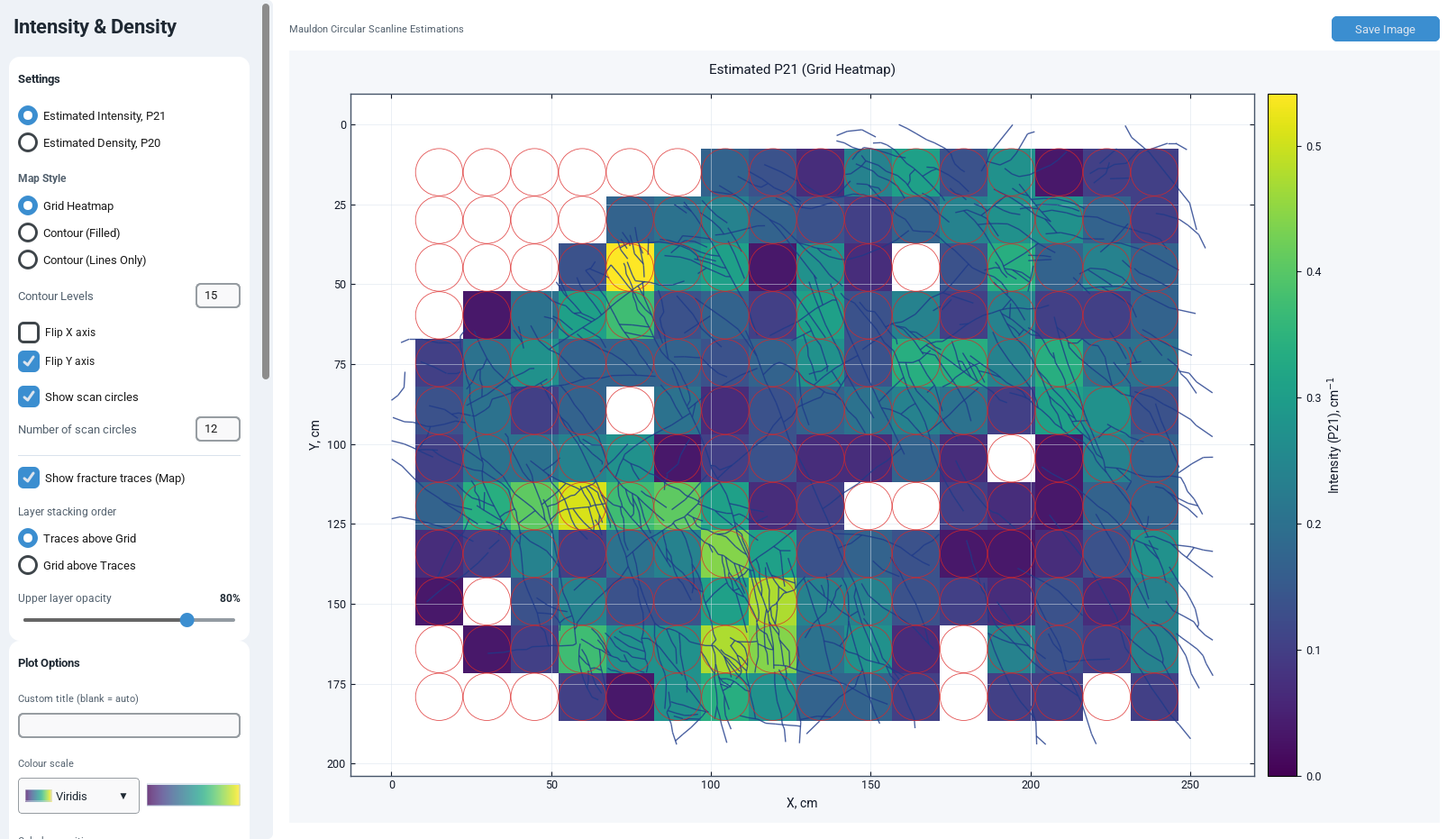
Show scan circles	Checkbox	show_circles_var	False	Overlays every individual scan‑circle boundary (unfilled, thin red outline) on the plot so the user can visually verify grid coverage and circle radius relative to fracture spacing.
Number of scan circles	Text entry	num_circles_var	"12"	Target circle count along the shorter map dimension; the algorithm (Section 6.1) derives the full 2‑D grid layout, spacing, and radius from this single value.
Show fracture traces (Map)	Checkbox	show_map_var	True	Toggles the LineCollection overlay of the raw fracture segments on top of (or below) the intensity/density surface.
Traces above Grid / Grid above Traces	Radio button pair	layer_order_var	"traces_top"	Sets the Z‑order and, correspondingly, which layer receives the partial‑opacity blend from the slider below (see Section 4.1.1).
Upper layer opacity	Slider (0.1–1.0)	top_opacity_var	0.8	Alpha applied to whichever layer (traces or grid) is currently on top per Layer stacking order; the lower layer remains fully opaque. Debounced via a 100 ms after() timer to avoid re‑triggering the (potentially expensive) kriging step on every pixel of slider drag.

4.1.1 Layer Stacking and Opacity Logic

The two overlay layers — the coloured intensity/density surface ("grid") and the fracture‑trace LineCollection ("traces") — are drawn with fractional Matplotlib z‑order values (1.5 and 2.5, or 2.5 and 1.5, depending on layer_order_var) chosen so that whichever layer the user places "on top" always renders above the other while both remain safely below axis text (z‑order 3.0) and above the canvas background (z‑order 1.0). The opacity slider always applies to the top layer only; the bottom layer is always drawn at alpha = 1.0, ensuring the underlying layer is never washed out regardless of which is chosen as primary.

4.2 Plot Options Card

Control	Widget	Variable	Default	Effect
Custom title (blank = auto)	Text entry	title_var	""	Overrides the automatically generated plot title (e.g. "Estimated P21 (Grid Heatmap)") with user‑supplied text when non‑empty.
Colour scale	Custom dropdown (CustomColorDropdown)	cmap_var / _cmap_resolved	"Viridis"	Selects the Matplotlib colormap applied to the heatmap/contour fill. A 104×28 px live gradient swatch previews the selected colormap. Internally resolved to a matplotlib colormap id (or the bundled Parula approximation) and cached in _cmap_resolved to avoid re‑parsing the display name on every redraw.
Colorbar position	Dropdown	colorbar_pos_var	"Right"	Bottom / Top / Left / Right / None — passed to Matplotlib's fig.colorbar(..., location=...). Selecting None suppresses colour‑bar rendering entirely.

4.3 Map Elements Card

Control	Variable	Default	Effect
Outer BG	outer_bg_var	#F5F7FA	Colour of the Matplotlib Figure background, outside the plot axes.
Plot BG	inner_bg_var	#FFFFFF	Colour of the Axes background (i.e. inside the plot frame).
Grid Color	grid_color_var	#D9E2EC	Colour of the reference grid lines (only drawn when "Show grid lines" is checked).
Trace Color	trace_color_var	#1E3A8A	Colour of the fracture‑trace LineCollection overlay.
Contour Line Color	contour_line_color_var	#000000	Colour of contour isolines (and their inline numeric labels) in either contour rendering style.
Show grid lines	grid_var	True	Toggles ax.grid() with the configured colour and 0.6 alpha.
Show scale	show_scale_var	False	Toggles a data‑accurate scale bar in the lower‑right of the map — see Section 4.3.1.
Scale Color	scale_color_var	#1F2933	Colour used to draw the scale bar (and its label/ticks).
Scale style	scale_style_var	"Solid bar"	Chooses how the scale bar is rendered — Solid bar (single filled block), Segmented bar (alternating filled/unfilled quarters), or Ticked line (a plain line with end ticks and no fill).
Border Color	border_color_var	#475569	Colour applied to all four Matplotlib Axes spines.
Border Width	border_width_var	"1.0"	Line width (points) applied to all spines; invalid entries silently fall back to 1.0.
Contour Line Width	contour_line_width_var	"0.5"	Line width used for contour isolines; invalid entries fall back to 0.5.

4.3.1 Scale Bar Rendering (_add_intensity_scale_bar)

When "Show scale" is enabled, _add_intensity_scale_bar() adds a data‑accurate mpl_toolkits.axes_grid1.anchored_artists.AnchoredSizeBar anchored to the lower‑right corner of the map (loc="lower right"). The bar's physical length is chosen by a "nice number" heuristic — the largest value of the form 1, 2, or 5 × 10ⁿ that does not exceed 22% of the current X‑axis span — so the labelled length is always a round, easily read figure rather than an arbitrary fraction of the map width.

The bar's label automatically converts units: if the project's display unit is metres and the computed bar length is 1000 or greater, the label is shown in kilometres (e.g. "2 km") instead of an unwieldy metre value (e.g. "2000 m"); for any other unit, or a length under 1000 m, the label uses the display unit unchanged. The three "Scale style" options are all drawn from the same underlying bar: Solid bar leaves the default filled rectangle as‑is; Segmented bar hides that rectangle and rebuilds it as four alternating filled/unfilled quarter‑segments in the chosen scale colour and the Plot BG colour; Ticked line suppresses the vertical bar height entirely, leaving only the horizontal line and its end ticks.

4.4 Background Image Card

This card lets the user overlay a georeferenced field photograph or outcrop image beneath the intensity/density surface, exactly mirroring the equivalent controls on the Fracture Map, Connectivity, and Profile Cross‑section tabs, so that a single calibrated image can be reused across every spatial tab in the Static Analyzer without re‑uploading it.

Control	Widget	Variable	Behaviour
Show real photo behind plot	Checkbox	p21_bg_mode_var	On check, calls _resolve_p21_bg_image_path(prompt_if_missing=True), which first tries to auto‑detect an already‑known image (this tab's own path, the Fracture Map tab's calibrated image, or the <svg_base>_bg.png sidecar written by the Trace Map tool) before opening a file‑browse dialog; if no image can be resolved, the checkbox is reset to unchecked.
Change Image…	Button	—	Opens a file dialog restricted to common raster formats (PNG, JPG/JPEG, BMP, TIFF, WEBP) and stores the chosen path.
Status label	Read‑only label	—	Displays "Image: <basename>" when a valid path is set, or "No image set" otherwise.
Image opacity (0–1)	Text entry	p21_bg_alpha_var	Default 1.0. Alpha blended into ax.imshow(); values are clamped to [0, 1] before use.

The image is drawn with ax.imshow(extent=(xMin, xMax, yMax, yMin), origin='upper', zorder=0), which intentionally swaps the vertical extent bounds to compensate for the SVG/screen convention of Y increasing downward — matching the same fix applied consistently across every other spatially‑aware tab in the application (Fracture Map, Connectivity, Profile Cross‑section).

4.5 Global Results Card (Read‑Only)

Field	Meaning
Grid Layout (X x Y)	The resolved scan‑circle grid dimensions, xNumCircle × yNumCircle, after the packing algorithm in Section 6.1 has run.
Total Scan Circles	xNumCircle × yNumCircle, the total number of circular sampling windows used.
Global Intensity (P21)	The single scalar network‑wide intensity, total fracture length divided by mapped area, with a unit⁻¹ superscript matching the active display unit.
Global Density (P20)	The single scalar network‑wide density, trace count (df["Trace"].nunique()) divided by mapped area, with a unit⁻² superscript. It is deliberately not a segment count: reporting len(lengths) here would make the density scale with digitisation density, so a 40‑trace network drawn with ten segments per trace would read ten times too high.

5. Mathematical Background

The circular scanline method was developed to overcome a fundamental limitation of straight‑line scanlines: the number of fracture intersections recorded by a straight scanline is systematically biased against fractures that are sub‑parallel to the scanline direction (the well‑known Terzaghi orientation bias (Terzaghi, 1965; Priest, 1993)). A circular sampling window, having no preferred direction, removes this bias, provided fracture intensity is evaluated using the correct geometric estimator (Mauldon, 1998; Mauldon et al., 2001). Comparative appraisals of outcrop sampling schemes consistently find the circular-window family to be the least biased of the practical alternatives (Zeeb et al., 2013; Watkins et al., 2015).

5.1 Symbol Definitions

Symbol	Description	Units
r	Radius of a circular scan window (rCircle in the implementation).	[length]
N	Number of discrete fracture‑segment/circle‑boundary intersection points found for one scan circle.	count
M	Number of fracture trace tips that fall strictly inside a scan circle. A tip is the first point of a trace's first segment or the last point of its last segment; interior polyline vertices are not tips and are excluded by _trace_tip_masks().	count
I	Local (per‑circle) estimate of P21, fracture intensity.	[length]⁻¹
D	Local (per‑circle) estimate of P20, fracture density.	[length]⁻²
L_tot	Sum of all segment lengths in the mapped dataset (Σ Length_m).	[length]
n_traces	Number of distinct traces in the mapped dataset, df["Trace"].nunique(). Not the segment count.	count
A_map	Bounding‑box area of the mapped dataset, (x_max−x_min)×(y_max−y_min).	[length]²

5.2 Circle‑Based P21 (Intensity) Estimator

For a single scan circle of radius r, the Mauldon circular‑scanline estimator of areal fracture intensity is:

This relationship follows from integral‑geometry (Buffon‑type) arguments relating the expected number of crossings of a fracture network with the boundary of a convex sampling window to the total trace length enclosed, and holds regardless of the internal orientation distribution of the fractures — which is precisely why the method is orientation‑unbiased (Mauldon, 1998). In the implementation, N corresponds to N_circle, the count of valid line‑segment/circle‑boundary root crossings (Section 6.2), and I corresponds to one entry of the I_grid array. In the P_ij notation of Dershowitz and Herda (1992) this quantity is P21: one‑dimensional features (trace length) measured over a two‑dimensional region.

5.3 Circle‑Based P20 (Density) Estimator

The companion density estimator counts fracture trace tips falling inside the circle:

where M is the number of trace tips inside the window (Mauldon et al., 2001, §2). This is coded as M_circle / (2 * π * rCircle**2). The normalisation constant is 2πr², not the naive πr², because a trace contributes two tips: for a tip density of 2d per unit area over a window of area πr², the expected count is E[M] = 2d·πr², so the unbiased estimate of the trace density d is M/(2πr²). Dividing the two estimators returns the Mauldon mean trace length,

which is exactly the mean‑length estimator published alongside them (Mauldon, 1998; Rohrbaugh et al., 2002), so the constants are not free parameters that could be adjusted.

5.4 Global (Network‑Wide) Statistics

In addition to the spatially resolved I_grid/D_grid arrays, the tab reports two single‑value statistics computed directly from the full dataset rather than by averaging the per‑circle grid, giving an estimate that is insensitive to grid resolution or circle placement:

These are the classical, non‑circular definitions of areal intensity and density applied to the entire bounding box of the dataset, and are what is displayed in the Global Results card.

5.5 Scan‑Circle Packing Geometry

Given a user‑specified target circle count n (num_circles_var) and the data's bounding‑box dimensions Δx = x_max−x_min and Δy = y_max−y_min, the algorithm computes a near‑tangent, non‑overlapping rectangular grid of circles. Denoting the longer of Δx, Δy as the "primary" axis (n circles are placed along it) and the shorter as the "secondary" axis:

The 0.99 scale factor intentionally shrinks each circle by 1% relative to exact tangency, preventing floating‑point edge cases in which adjacent circles would otherwise touch or micro‑overlap. When Δx equals Δy exactly, both axes use n circles directly with spacing based on the smaller of the two per‑axis spacings. Circle centres are then placed at:

producing a regular grid of centres based on the data's bounding box, not a mapped-area polygon. This does not guarantee that every circle lies inside the surveyed domain, especially for irregular coverage or a narrow domain where the secondary circle count is clamped to one. Inspect coverage with Show scan circles enabled.

6. Algorithms and Internal Workflow

_draw_trace_intensity() is the single entry point that orchestrates data validation, grid construction, the vectorised geometric intersection test, statistic computation, and Matplotlib rendering, in that order, every time any control changes. This section walks through that pipeline in the sequence it executes.

6.1 Step 1 — Validation and Grid Layout

1. Verify self.results is non‑empty and, if the data source is Excel, that the segments carry real spatial geometry (not orientation‑only preset strike/dip data).
2. Verify the five required columns (X1, Y1, X2, Y2, Length_m) are present.
3. Parse num_circles_var and contour_levels_var from their text fields, applying documented fallback defaults (12 and 15 respectively) on parse failure, and writing the corrected/parsed value back into the StringVar so the sidebar reflects what was actually used.
4. Compute the dataset bounding box (xMin, xMax, yMin, yMax) from the min/max of both endpoint columns, and derive Δx, Δy (mapArea = Δx × Δy).
5. Apply the packing geometry of Section 5.5 to obtain xNumCircle, yNumCircle, rCircle, and the two per‑axis centre‑spacing increments, clamping both circle counts to a minimum of 1.
6. Build the 1‑D centre coordinate arrays x_centers, y_centers and combine them into a 2‑D meshgrid (CX, CY), which is then flattened to CX_flat, CY_flat for the vectorised intersection step.

6.2 Step 2 — Vectorised Line‑Circle Intersection Test

Rather than looping over every (segment, circle) pair in Python, the module builds two broadcastable NumPy arrays — one of shape (n_segments, 1) for the segment endpoints and one of shape (1, n_circles) for the circle centres — so that every pairwise combination is evaluated simultaneously via NumPy broadcasting. For each segment i and circle k, the standard parametric line/circle intersection is solved:

A real root t is a genuine crossing of the (infinite) circle by the segment only if 0 ≤ t ≤ 1 (i.e. the crossing lies within the finite segment, not its extension) and Δ ≥ 0. The implementation additionally guards against degenerate zero‑length segments (a = 0) by substituting a = 1 for those rows before division and separately masking them out via the boolean array valid = a > 0, so no division‑by‑zero warning is ever raised. The second root is only counted as distinct when t1 ≠ t2 (t_valid2 additionally requires t1 != t2), preventing a tangent intersection from being double‑counted.

Per scan circle, the intersection count N (summed over all segments, over the segment axis) becomes N_circle. The two "endpoint inside circle" tests d₁_sq < r² and d₂_sq < r² (squared distance from each of the segment's two endpoints to the circle centre, compared against r²) are each AND‑ed with a trace‑tip mask before summing:

so that M_circle is a count of genuine trace tips, not of segment endpoints (Section 5.3). _trace_tip_masks() groups the rows by Trace, orders each group by Segment, and sets tip1 True on the first row of the trace and tip2 True on its last; every other endpoint is an interior polyline vertex and stays False. If the frame carries no Trace column the helper degrades gracefully by treating every row as its own trace (both masks all True), which reproduces the older segment‑endpoint behaviour only in the one case where it is correct.

Both N_circle and M_circle are reshaped from a flat (n_circles,) vector back into the 2‑D (yNumCircle, xNumCircle) grid shape matching CX, CY, so that I_grid and D_grid (per Section 5.2–5.3) can be plotted directly with pcolormesh or used as scattered input to the kriging/interpolation step.

6.3 Step 3 — Global Statistics and Sidebar Update

total_length = Σ(Length_m), mapArea, n_traces = int(df["Trace"].nunique()), global_P21, and global_P20 are computed per 5.4 and pushed into the four Global Results labels, alongside the resolved grid layout (xNumCircle × yNumCircle) and total scan‑circle count. When the frame has no Trace column, n_traces falls back to len(lengths), i.e. one trace per row. The unit suffix (m, cm, mm, or km) is read live from the shared _static_map_unit_var so the displayed units always track the workspace's current display unit.

6.4 Step 4 — Rendering Dispatch

Based on plot_style_var, one of three rendering branches executes:

6.4.1 Heatmap

The active grid (I_grid or D_grid, selected by plot_mode_var) is masked wherever its value is exactly zero (np.ma.masked_where) so empty regions render as fully transparent rather than as a spurious colour at the bottom of the colour scale, and drawn with ax.pcolormesh() over cell‑edge coordinate arrays derived by expanding each centre by ±half the corresponding axis spacing.

6.4.2 Contour (Filled) / Contour (Lines Only)

Both contour styles first interpolate the sparse per‑circle grid values onto a dense 100×100 regular mesh spanning the full bounding box. Two interpolation paths are supported:

• Ordinary Kriging (preferred) — if the pykrige package is available, an OrdinaryKriging model with a linear variogram (slope = 1.39096×10⁻⁸, nugget = 0.0) is fit to the scan‑circle centres and evaluated on the dense grid via OK.execute('grid', …), with negative kriged values clipped to zero (fracture intensity/density cannot be negative).
• Cubic griddata fallback — if pykrige is not installed, or kriging raises an exception, scipy.interpolate.griddata(…, method='cubic', fill_value=0) is used instead, silently degrading gracefully rather than failing the redraw.

Contour levels are computed with Matplotlib's MaxNLocator when contour_levels_var parses to an integer count, or as a fixed step interval (np.arange) when the parsed value is a non‑integer float, allowing the user to request either "n bands" or "a contour every X units" behaviour from the same text field. A second, level‑filtered array with the zero level removed (plot_levels_lines) is used specifically for the isoline/label pass, so a spurious "0.000" contour is never drawn or labelled in the interior of the map, while the zero level is still retained in the filled‑colour pass (plot_levels_fill) so the colour scale correctly represents zero‑intensity regions.

For the "Contour (Filled)" style, ax.contourf() draws the shaded bands at 0.85× the layer alpha; for both contour styles, ax.contour() draws black (or user‑coloured) isolines with inline numeric labels via ax.clabel(inline=True, fontsize=8, fmt='%.3f').

6.5 Step 5 — Overlay Layers, Axis Styling, and Colour Bar

After the primary surface is drawn, the module conditionally adds: the fracture‑trace LineCollection (if Show fracture traces is checked), the individual scan‑circle outlines (if Show scan circles is checked), and the background photograph (if enabled), respecting the z‑order/opacity rules of Section 4.1.1. Axis limits are padded by 5% of each dimension, aspect is fixed to 'equal', axis flips are applied, grid lines and border/spine styling are applied from the Map Elements card, and the scale bar is added last via _add_intensity_scale_bar() (see Section 4.3.1) so it sits above every other map layer. Finally fig.tight_layout() and _align_colorbar_to_plot() commit the layout before canvas.draw_idle() renders the frame; the same tight‑layout/alignment pair is re‑run independently by the canvas layout‑sync handler described in Section 2.3 whenever the tab is resized or first shown.

6.6 Caching and Performance Optimisation

Kriging (and, to a lesser extent, cubic griddata interpolation) is computationally the most expensive step in the pipeline, particularly for large scan‑circle grids. To avoid re‑running it on every purely cosmetic redraw (e.g. a colour change), the module maintains a single‑entry cache, self._krige_cache, keyed on a tuple of (len(df), loaded file path, plot_mode, num_circles_var) — i.e. the inputs that actually influence the interpolated surface. On each contour‑style redraw, the current key is compared against the cached key; if they match, the previously computed fine_Z array is reused directly, and kriging/griddata is skipped entirely. Any change to the underlying data, the selected statistic (P21 vs P20), or the requested circle count invalidates the cache and forces recomputation.

The opacity slider additionally uses a 100 ms after() debounce (self._opacity_timer) so that dragging the slider does not trigger a full recomputation (including a potential kriging pass) on every intermediate pixel value emitted during the drag; only the final settled value (100 ms after the last movement) triggers _draw_trace_intensity().

The core intersection test itself (Section 6.2) is implemented purely with NumPy array broadcasting rather than nested Python loops, so its cost scales as O(n_segments × n_circles) in vectorised array operations rather than in interpreted Python iterations — a substantial performance benefit for networks with hundreds to thousands of segments sampled by tens of circles.

7. Statistical Methods

7.1 Point Estimators vs. Grid Interpolation

The tab distinguishes between two distinct statistical operations: (1) unbiased point estimation of P21/P20 at each discrete scan‑circle location using the Mauldon estimators of Section 5.2–5.3, and (2) spatial interpolation between those discrete point estimates for continuous‑surface visualization (heatmap cell shading is a nearest‑value/no‑interpolation display of the raw grid, whereas the contour styles interpolate). Users should be aware that the interpolated contour surface between scan‑circle centres is a smoothed visual aid, not itself a rigorously unbiased estimator at arbitrary intermediate locations — the rigorous estimate exists only at the discrete circle centres.

7.2 Ordinary Kriging

When available, Ordinary Kriging is used for its property of exact interpolation at data points combined with a principled treatment of spatial autocorrelation via the fitted linear variogram model (Cressie, 1993; Chilès and Delfiner, 2012). A linear variogram was selected as a robust, parameter‑light default appropriate for scan‑circle sampling grids of moderate size, avoiding the need for interactive variogram model selection within the GUI. Because the variogram parameters are fixed rather than fit adaptively to each dataset, users working with strongly clustered or highly heterogeneous fracture intensity fields should treat the kriged surface as a qualitative smoothing aid rather than a geostatistically rigorous best linear unbiased predictor.

7.3 Cubic Spline Fallback

In the absence of PyKrige, scipy.interpolate.griddata with method='cubic' provides a smooth, differentiable interpolation surface (Virtanen et al., 2020). Cubic griddata does not honour the nugget/nugget‑free distinction of kriging and can produce mild over/undershoot (Gibbs‑like ringing) near sharp gradients in the underlying scan‑circle values; this is an accepted trade‑off for environments without the optional PyKrige dependency.

7.4 Global vs. Local Statistics — Interpretation Guidance

The Global Results panel's P21/P20 values are computed directly from the full dataset (total length, and total trace count, each divided by the bounding‑box area) and therefore represent the exact areal intensity/density of the digitized network over its full extent — they are not themselves circular‑scanline estimates and carry no orientation‑bias correction, but they also carry no scan‑circle sampling error, since they use every available data point. The gridded/contoured map, by contrast, reveals spatial heterogeneity in intensity/density that the single global value necessarily conceals; a network can have a modest global P21 while containing localized high‑intensity damage zones clearly visible on the map.

8. Visualization Components

Element	Matplotlib Object	Description
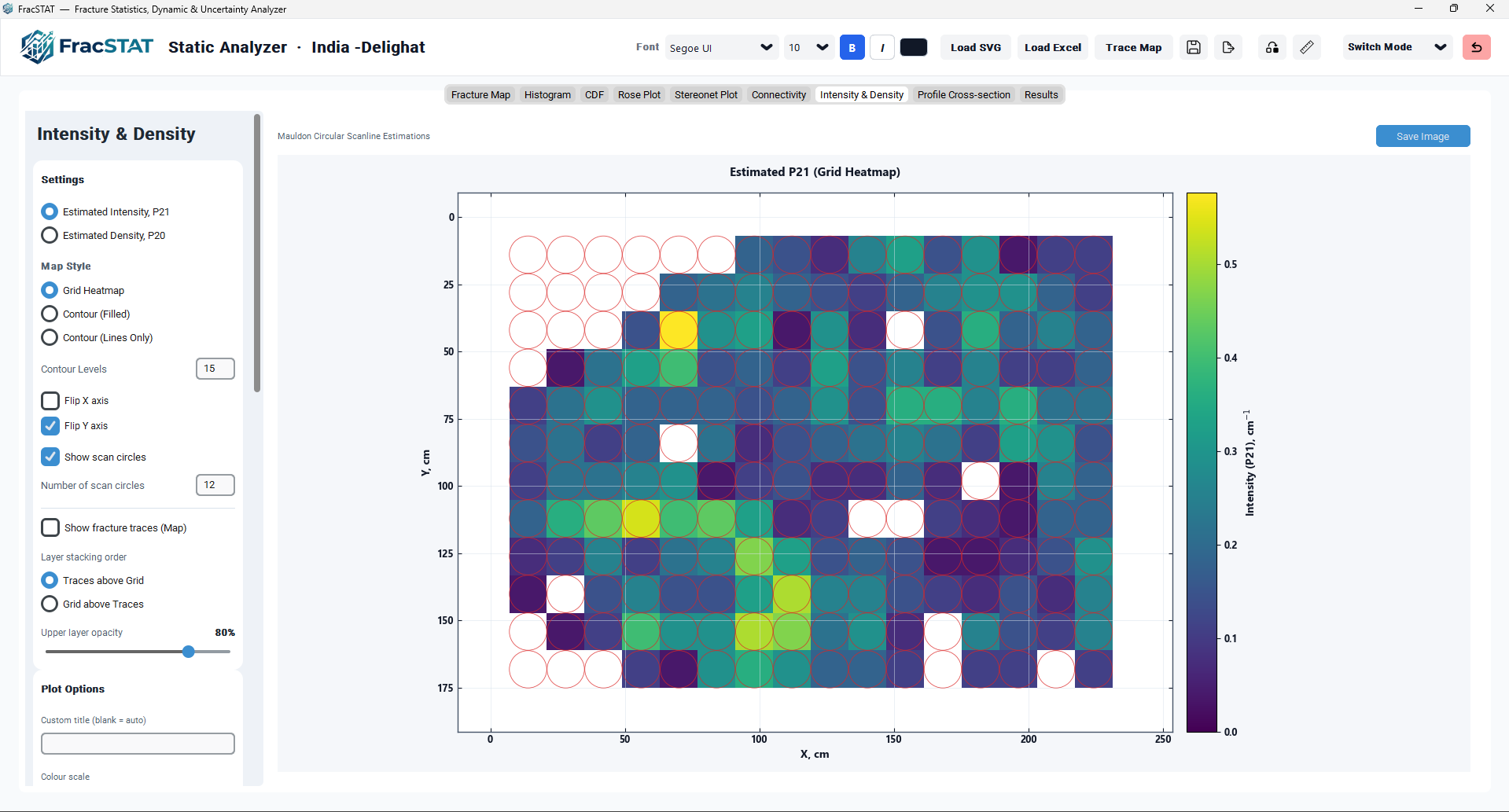
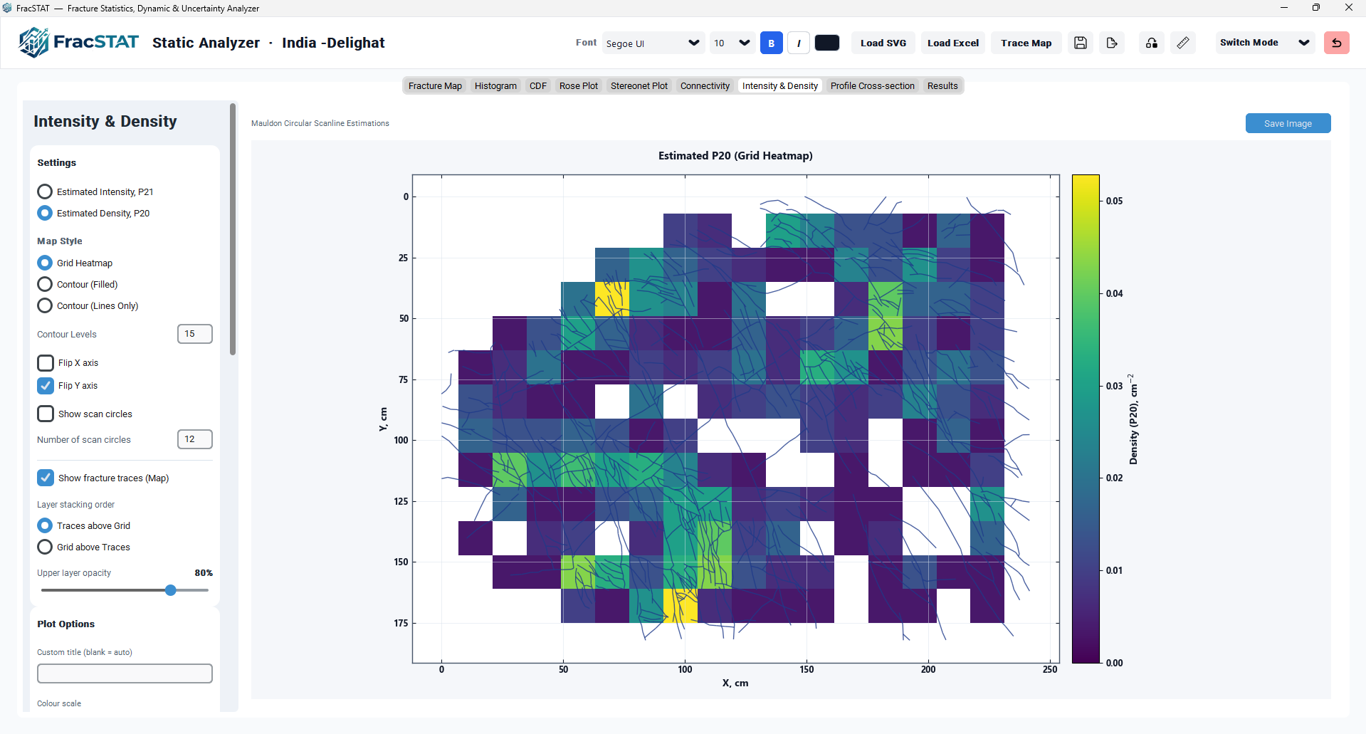
Heatmap surface	ax.pcolormesh()	Discrete, cell‑based colouring of the raw (non‑interpolated) I_grid/D_grid values, masked where zero.
Filled contour	ax.contourf()	Smooth, kriged/interpolated shaded bands of the selected statistic.
Contour isolines	ax.contour() + ax.clabel()	Labelled black (or user‑coloured) contour lines, always available in both contour styles, and independently controllable in width/colour.
Fracture trace overlay	matplotlib.collections.LineCollection	All digitized fracture segments drawn as a single vectorised line collection for performance, coloured per Map Elements > Trace Color.
Scan‑circle outlines	matplotlib.patches.Circle (unfilled)	One outline per scan‑circle centre, only drawn when "Show scan circles" is enabled; useful for auditing grid coverage and spacing.
Background photograph	ax.imshow()	Optional calibrated field photo drawn beneath (z‑order 0) all data layers.
Scale bar	mpl_toolkits.axes_grid1.anchored_artists.AnchoredSizeBar	Optional data‑accurate scale bar anchored to the lower‑right of the map, drawn last (above all other layers); see Section 4.3.1.
Colour bar	fig.colorbar(mappable, ax=ax, location=…)	Attached via Matplotlib's axis‑anchored colorbar API, but its final position, width, and axes locator are explicitly overridden by the custom _align_colorbar_to_plot() method to keep it thin and flush against the map rather than leaving Matplotlib's default (and often oversized) empty band beside it. Its tick formatter also has set_scientific(False) and set_useOffset(False) applied, so intensity/density values are always shown as plain decimal numbers instead of scientific notation or an offset.

Figure 8.1 — Example heatmap rendering of P21 intensity across a mapped fracture network, with scan circles overlaid and fracture traces drawn above the grid at 80% opacity.

Figure 8.2 — Example kriged filled‑contour rendering of P20 density, showing labelled isolines and a right‑hand colour bar.

All text elements (titles, axis labels, colour‑bar labels, tick labels) are rendered using the workspace's currently selected font family, size, weight, and colour, which are applied globally via Matplotlib's rcParams by the shared _apply_workspace_font() mechanism common to every Static Analyzer tab — changing the font in the workspace header therefore updates this tab's plot text on the next redraw without any tab‑specific font code.

9. Advanced Features

9.1 Layer Stacking with Independent Opacity

The traces‑above‑grid / grid‑above‑traces toggle, combined with the single shared opacity slider, allows the user to visually emphasise either the raw fracture network (useful when validating that the intensity surface correctly reflects the underlying digitised traces) or the interpolated intensity/density field (useful for presentation‑quality figures where the traces would otherwise visually clutter a smooth contour surface).

9.2 Background Photograph Auto‑Detection

_autodetect_p21_bg_image_path() implements a three‑tier fallback search: (1) the path already stored in this tab's own p21_bg_image_path_var, if it still exists on disk; (2) the Fracture Map tab's calibrated background image path (_static_map_bg_image_path_var), letting a single calibration performed once on the main map propagate automatically to this tab; (3) the <svg_base>_bg.png sidecar file written automatically by the Trace Map tracing tool (tracer.py) whenever a background reference photo was used during digitisation. This layered lookup means most users will never need to manually browse for an image on this tab at all.

9.3 Adaptive Contour Level Specification

The Contour Levels field accepts either an integer (interpreted as a target band count, resolved via Matplotlib's MaxNLocator to "nice" round‑number boundaries) or a decimal value (interpreted as a fixed absolute contour interval in the data's own units, e.g. entering 0.05 draws contours every 0.05 units of P21). This dual behaviour is detected automatically from whether the parsed float has a zero fractional part.

9.4 Zero‑Level Suppression on Contour Labels

Because scan circles containing no fracture length and no trace tips correctly evaluate to I = 0 or D = 0, an unfiltered contour pass would frequently draw and label a "0.000" contour threading through every low‑intensity region of the map, adding visual noise without informative content. The implementation filters this level out of the isoline/label pass (plot_levels_lines) while retaining it in the colour‑fill pass (plot_levels_fill), so the zero‑intensity colour band is still shown, but not needlessly outlined and numerically labelled.

10. Performance Optimization

Because scan‑circle count enters the intersection test as a multiplicative factor on cost, users working with very dense fracture networks (many thousands of segments) are advised to keep the Number of scan circles control modest (10–20) unless finer spatial resolution is specifically required, since both the O(n_segments × n_circles) intersection test and, for contour styles, the kriging/interpolation step scale with the number of scan circles.

Technique	Where Applied	Benefit
Full vectorisation (NumPy broadcasting)	Line/circle intersection test (Section 6.2)	Avoids an explicit Python double loop over every (segment, circle) pair; scales efficiently to networks with thousands of segments.
Single‑entry kriging/interpolation cache	Contour rendering branch (Section 6.6)	Skips the most computationally expensive step (kriging or cubic griddata) whenever only cosmetic settings (colour, title, borders, etc.) have changed.
Debounced opacity slider	Layer opacity control	Prevents dozens of redundant full redraws (including potential re‑kriging) while a slider is actively being dragged; only the settled value triggers computation.
Colormap‑name resolution caching	_resolve_cmap() / _cmap_resolved	Avoids repeated dynamic imports and string‑matching lookups of the active colormap on every redraw once the dropdown has fired once.
Masked‑array rendering	Heatmap style	np.ma.masked_where() lets Matplotlib skip drawing (and colour‑mapping) cells with no data, reducing rendering overhead and avoiding a misleading colour for zero‑intensity cells.

11. Practical Examples

11.1 Example 1 — Assessing Fracture‑Damage Localisation

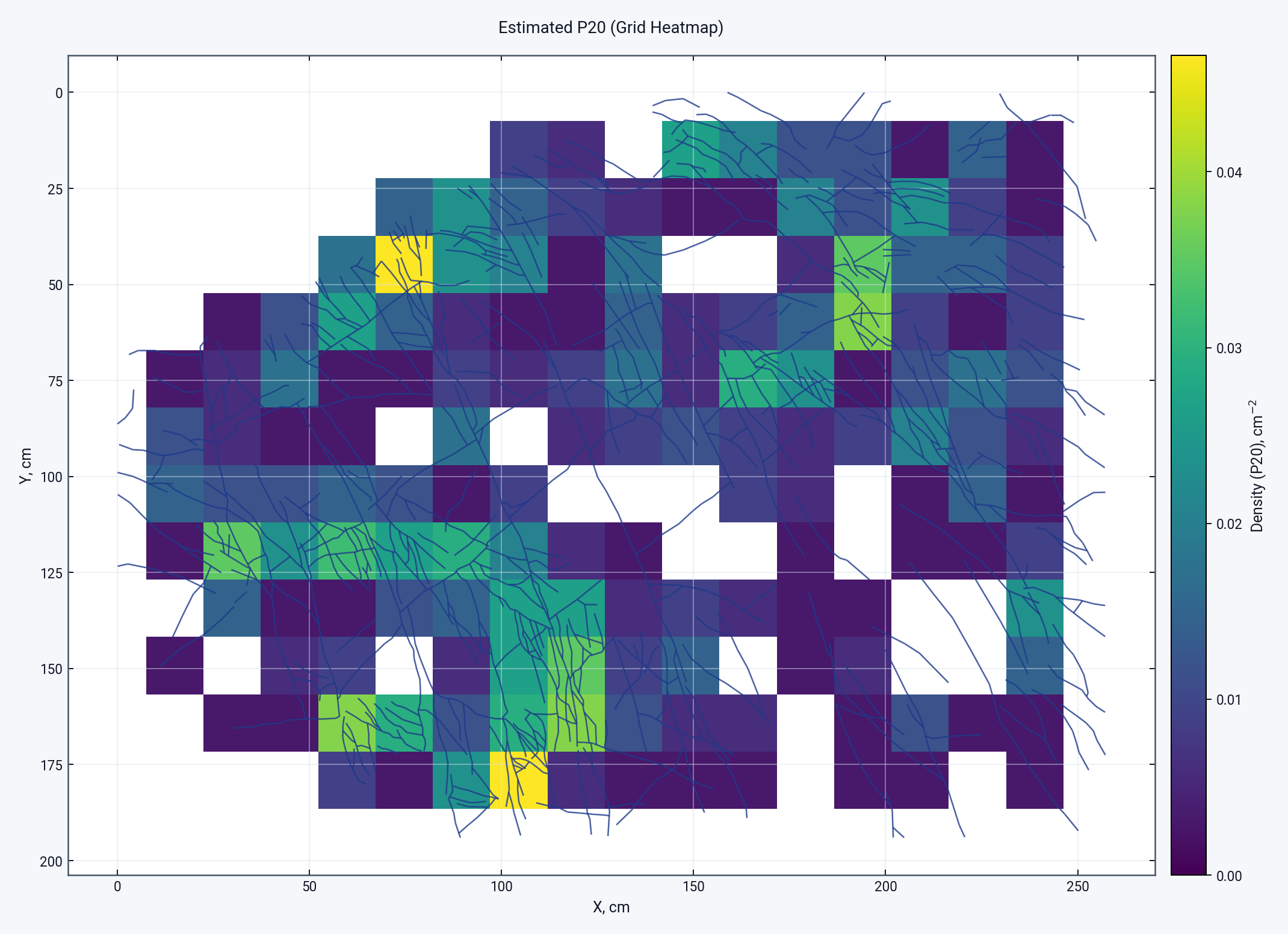
A user has digitised a fracture trace map from an outcrop photograph showing a fault damage zone. After loading the SVG on the Fracture Map tab, they switch to Intensity & Density, select Estimated Intensity (P21), choose Grid Heatmap for an immediate, uninterpolated view of local intensity, and increase Number of scan circles to 20 to resolve the damage‑zone boundary more sharply. The heatmap reveals a clear high‑P21 corridor coincident with the mapped fault trace, while the Global Results card reports a single average P21 for the whole outcrop — illustrating why the spatial map, not the global statistic alone, is needed to identify localized damage.

11.2 Example 2 — Publication‑Quality Kriged Density Map

For a manuscript figure, the user switches Plot Mode to Estimated Density (P20), Plot Style to Contour (Filled), sets Contour Levels to 12, enables the background field photograph at 40% opacity to provide geological context, sets Layer stacking order to Grid above Traces so the smooth kriged surface is the dominant visual element, and exports the figure via Save Image at the project's configured export DPI.

11.3 Example 3 — Comparing Circular‑Scanline vs. Global Statistics

A user wants to check whether their fracture network is spatially homogeneous. They record the Global Intensity (P21) value from the Global Results card, then visually inspect the heatmap for regions markedly brighter or darker than that global value. Large, spatially coherent deviations from the global mean indicate a network that should not be treated as areally stationary for downstream flow or geomechanical modelling; near‑uniform colouring across the map supports a stationarity assumption.

12. Geological Interpretation

Fracture intensity (P21) and density (P20) are foundational inputs to discrete fracture network (DFN) modelling, fractured‑reservoir permeability estimation, rock‑mass classification (e.g. RQD‑related indices), and slope‑stability or excavation‑damage assessments. Their spatial variability, as revealed by this tab's gridded/contoured maps, has direct engineering and geological significance:

• High‑P21 corridors frequently mark active or reactivated fault zones, relay ramps, or fold‑hinge damage zones where strain has been concentrated, and are commonly zones of enhanced permeability in naturally fractured reservoirs.
• Elevated P20 without a correspondingly high P21 can indicate a population of short, closely spaced fractures (e.g. from hydraulic shattering or thermal cracking) rather than a few long, throughgoing structures — an important distinction for connectivity and flow‑pathway modelling.
• Spatially uniform P21/P20 across a mapped domain supports treating the domain as statistically homogeneous for upscaling purposes, whereas strong local heterogeneity (as visualised here) motivates domain sub‑division or the use of spatially variable DFN input statistics.
• Because the circular‑scanline estimator is explicitly designed to be orientation‑unbiased, P21/P20 values computed here are more directly comparable between outcrops or map sheets with different structural trends than values derived from straight‑line scanlines oriented arbitrarily with respect to the dominant fracture set (Terzaghi, 1965; Zeeb et al., 2013).
• Both P21 and P20 are scale‑dependent quantities in a fractal or power‑law fracture population: the value obtained depends on the resolution at which traces were digitised and on the size of the sampling window, so comparisons between data sets are only meaningful at a matched observation scale (Ortega et al., 2006).

Users should bear in mind that all statistics in this tab are 2‑D, trace‑map‑derived measures; they characterise the exposed (or digitised) fracture trace pattern on a mapped surface (an outcrop face, a satellite image, or a core photograph laid flat) and are not automatically equivalent to volumetric (3‑D) fracture intensity (P32) without additional geometric assumptions relating trace‑plane sampling to the true 3‑D fracture population — a conversion that FracSTAT's Static Analyzer does not perform in this tab, and which requires assumptions about the fracture size and orientation distributions (Zhang and Einstein, 2000).

13. Implementation Notes

Topic	Note
Class and inheritance	TraceIntensityTab is implemented as a mixin class, combined with several sibling mixins (StaticMapTab, StaticLengthsTab, StaticCDFTab, StaticAnglesTab, StaticStereonetTab, StaticFluidFlowTab, StaticGraphsTab, StaticResultsTab, WorkspaceHeaderMixin) into the single StaticAnalyzerApp class, following the shared‑mixin architecture used throughout the Static Analyzer.
Shared data source	self.results / self._static_results is populated exclusively by the Fracture Map tab's geometry pipeline (run_static_calculations(), overridden at runtime to _static_map_run_geometry()); this tab performs no independent geometry computation of its own beyond the scan‑circle grid and intersection test.
Colormap resolution helper	The module‑level _resolve_cmap() function is duplicated (by design, for decoupling) from the equivalent helper in static_map_tab.py; both resolve a display colormap name to a matplotlib Colormap object, including the app's custom bundled Parula approximation via SlipTendencyApp._parula_colormap().
Trace‑tip helper	The module‑level _trace_tip_masks(df) returns two row‑aligned boolean arrays marking which of each segment's two endpoints is a genuine trace tip (first row's X1/Y1 and last row's X2/Y2 within each Trace group, ordered by Segment). It is the single point at which the density estimator is made independent of digitisation density; the equivalent trace‑level logic on the Connectivity tab lives in core/branch_counter.py's _trace_tip_lookup().
Palette source	Default background/border/grid colours are seeded once from self.plot_palette() (a method shared across the workspace) at widget‑construction time, but thereafter are fully independent, user‑editable StringVars specific to this tab.
Unit propagation	The display unit (m/cm/mm/km) is never stored locally; it is read on every draw from the shared _static_map_unit_var owned by the Fracture Map tab, ensuring the Intensity & Density tab always reports statistics in the workspace's currently active unit even if the unit is changed after this tab was last drawn.
No independent SVG/Excel loading	This tab intentionally exposes no Load SVG / Load Excel controls; all data loading is centralized in the shared workspace header and the Fracture Map tab, per the application's overall data‑flow design.

14. Limitations

Limitation	Description
Tip‑based P20 estimator	The local P20 estimator counts trace tips inside each scan circle rather than trace centres. This is the published circular‑window estimator (Mauldon et al., 2001) and is digitisation‑invariant, since interior polyline vertices are masked out by _trace_tip_masks(). It remains a sampling estimator, however: a long trace crossing the window without terminating in it contributes no tips, so a single circle placed on a sparse, long‑trace network can read low while the global P20 does not. Compare the map against the Global Results value (Section 7.4) before treating a local minimum as real.
Bounding‑box sampling area	Both global statistics are normalised by the data's own bounding box, A_map = Δx × Δy, not by an independently chosen sampling window. Where the mapped domain is not rectangular, or where traces do not reach the box edges, A_map overstates the true sampled area and both P21_global and P20_global are correspondingly biased low. The Connectivity tab, by contrast, accepts an explicit sampling window for exactly this reason.
Fixed variogram model	The fixed linear‑variogram kriging model (Section 7.2) is not adaptively fit to each dataset's own spatial autocorrelation structure; it functions as a general‑purpose smoothing interpolator rather than a geostatistically optimal predictor for every possible fracture network (Chilès and Delfiner, 2012). No kriging variance is reported, so the map carries no interpolation‑uncertainty estimate.
Indirect grid resolution control	Grid resolution is controlled indirectly, via the Number of scan circles field, which sets circle count along the shorter map dimension only — very elongated (high aspect‑ratio) datasets may produce an uneven number of circles along the two axes.
No confidence intervals on local estimates	Each per‑circle P21 and P20 value is a single count divided by a geometric constant, so its sampling error is inherently large for small N or M. No standard error, Poisson interval, or bootstrap confidence band is computed, and adjacent circles are treated as independent even where they nearly touch (Rohrbaugh et al., 2002).
Scale dependence not quantified	Results are reported at one circle radius only. Because P21 and P20 in a power‑law fracture population depend on observation scale (Ortega et al., 2006), no multi‑radius sweep or scaling exponent is produced, and values are not comparable across data sets digitised at different resolutions.
Circles are not clipped to the mapped domain	The packing geometry (Section 5.5) insets circle centres from the bounding box but does not guarantee that every circle lies wholly inside the digitised area. A circle overlapping unmapped ground records fewer crossings than it should and reads spuriously low; inspect coverage with Show scan circles enabled.

15. References

Sources are listed alphabetically within each group. In-text citations throughout this page link to the corresponding entry below.

15.1 Fracture Intensity and Circular-Window Sampling

• Dershowitz, W. S., & Herda, H. H. (1992). Interpretation of fracture spacing and intensity. In Proceedings of the 33rd U.S. Symposium on Rock Mechanics (pp. 757–766). Balkema, Rotterdam. — source of the P_ij notation; P20 is defined as the number of fractures per unit area.
• Mauldon, M. (1998). Estimating mean fracture trace length and density from observations in convex windows. Rock Mechanics and Rock Engineering, 31(4), 201–216. https://doi.org/10.1007/s006030050021
• Mauldon, M., Dunne, W. M., & Rohrbaugh, M. B. (2001). Circular scanlines and circular windows: new tools for characterizing the geometry of fracture traces. Journal of Structural Geology, 23(2–3), 247–258. https://doi.org/10.1016/S0191-8141(00)00094-8
• Ortega, O. J., Marrett, R. A., & Laubach, S. E. (2006). A scale-independent approach to fracture intensity and average spacing measurement. AAPG Bulletin, 90(2), 193–208. https://doi.org/10.1306/08250505059
• Rohrbaugh, M. B., Dunne, W. M., & Mauldon, M. (2002). Estimating fracture trace intensity, density, and mean length using circular scan lines and windows. AAPG Bulletin, 86(12), 2089–2104. https://doi.org/10.1306/61EEDE0E-173E-11D7-8645000102C1865D
• Zhang, L., & Einstein, H. H. (2000). Estimating the intensity of rock discontinuities. International Journal of Rock Mechanics and Mining Sciences, 37(5), 819–837. https://doi.org/10.1016/S1365-1609(00)00022-8

15.2 Sampling Bias and Survey Practice

• Priest, S. D. (1993). Discontinuity Analysis for Rock Engineering. Chapman & Hall, London. https://doi.org/10.1007/978-94-011-1498-1
• Terzaghi, R. D. (1965). Sources of error in joint surveys. Géotechnique, 15(3), 287–304. https://doi.org/10.1680/geot.1965.15.3.287
• Watkins, H., Bond, C. E., Healy, D., & Butler, R. W. H. (2015). Appraisal of fracture sampling methods and a new workflow to characterise heterogeneous fracture networks at outcrop. Journal of Structural Geology, 72, 67–82. https://doi.org/10.1016/j.jsg.2015.02.001
• Zeeb, C., Gomez-Rivas, E., Bons, P. D., & Blum, P. (2013). Evaluation of sampling methods for fracture network characterization using outcrops. AAPG Bulletin, 97(9), 1545–1566. https://doi.org/10.1306/02131312042

15.3 Geostatistics, Interpolation and Software

• Chilès, J.-P., & Delfiner, P. (2012). Geostatistics: Modeling Spatial Uncertainty (2nd ed.). John Wiley & Sons. https://doi.org/10.1002/9781118136188
• Cressie, N. A. C. (1993). Statistics for Spatial Data (Revised ed.). John Wiley & Sons. https://doi.org/10.1002/9781119115151
• Harris, C. R., Millman, K. J., van der Walt, S. J., Gommers, R., Virtanen, P., Cournapeau, D., … Oliphant, T. E. (2020). Array programming with NumPy. Nature, 585(7825), 357–362. https://doi.org/10.1038/s41586-020-2649-2
• Hunter, J. D. (2007). Matplotlib: A 2D graphics environment. Computing in Science & Engineering, 9(3), 90–95. https://doi.org/10.1109/MCSE.2007.55
• Virtanen, P., Gommers, R., Oliphant, T. E., Haberland, M., Reddy, T., Cournapeau, D., … van Mulbregt, P. (2020). SciPy 1.0: fundamental algorithms for scientific computing in Python. Nature Methods, 17(3), 261–272. https://doi.org/10.1038/s41592-019-0686-2