Static Profile Tab
Located at static_analyzer/tabs/static_profile_tab.py, the Profile
Cross-section tab (implemented as the mixin class StaticGraphsTab) provides
a one-dimensional sampling framework for extracting geometric and statistical fracture
attributes along, and perpendicular to, a user-defined reference line ("scan line") superimposed
on a digitized fracture-trace map. It lets a user interrogate spatial trends in fracture length,
orientation, spacing, and intensity across a mapped outcrop, drill-core photomosaic, or
remote-sensing image, in a manner analogous to a geological cross-section or transect survey.
This module digitizes the classical field scanline survey: a straight scanline is laid across
an outcrop and the fractures crossing it are logged together with their spacing, orientation,
and length, yielding a one-dimensional statistical sample of an otherwise two-dimensional
fracture network — the basis of fracture-intensity metrics such as P10, P21, and P20
(Priest, 1993;
Dershowitz and Herda, 1992). The module
operates exclusively within the Static Analyzer workspace, performing purely geometric analysis
with no dependency on stress, slip tendency, or any mechanical property computed in the Dynamic
Analyzer.
On this page
- 1. Position within the FracSTAT Architecture
- 2. Interface Overview
- 3. Data Input Requirements
- 4. Settings and Controls
- 5. Mathematical Background
- 6. Algorithms
- 7. Internal Workflow
- 8. Statistical Methods and Quantitative Outputs
- 9. Visualization Components
- 10. Advanced and Interactive Features
- 11. Performance Optimization
- 12. Practical Examples
- 13. Geological Interpretation
- 14. Implementation Notes
- 15. Limitations
- 16. References
Once a fracture-trace map has been imported into the Static Analyzer (via an SVG trace file or a spatial Excel/CSV coordinate table), the user positions a two-point reference line anywhere across the mapped area — either by typing coordinates or by clicking directly on the map — and the module computes, for every fracture segment or trace that the reference line crosses or lies near:
- The one-dimensional position ("distance along") at which each fracture intersects the line, together with the trace length, segment length, or segment angle associated with that intersection;
- The perpendicular offset ("distance from") of trace and segment midpoints relative to the line, again cross-plotted against trace length, segment length, or segment angle;
- A Mauldon-style circular-scanline estimate of fracture intensity (P21) and density (P20) evaluated at a user-specified number of positions along the line (Mauldon et al., 2001).
The module therefore serves two complementary purposes: it is a spatial-trend diagnostic tool, letting the user determine whether fracture attributes vary systematically across a mapped domain (for example, increasing intensity toward a fault zone), and it is a quantitative intensity/density estimator that is robust to network anisotropy, because the Mauldon circular-window method removes the orientation bias inherent in straight scanline counts (Terzaghi, 1965; Mauldon et al., 2001).
1. Position within the FracSTAT Architecture
FracSTAT is organised into two principal analytical workspaces — the Static Analyzer (geometric fracture-network characterisation) and the Dynamic Analyzer (stress-based slip/dilation tendency analysis) — plus a placeholder Uncertainty Analyzer workspace. The Static Analyzer itself is a tabbed workspace comprising nine tabs: Fracture Map, Histogram, CDF, Rose Plot, Stereonet Plot, Connectivity, Intensity & Density, Profile Cross-section, and Results.
The Profile Cross-section tab is implemented by the StaticGraphsTab mixin class,
combined via multiple inheritance into the StaticAnalyzerApp class alongside the
other eight tab mixins and the shared WorkspaceHeaderMixin top toolbar. All tabs
share the same underlying data source: a pandas DataFrame stored on the application instance as
self.results, which is (re)computed whenever an SVG or Excel/CSV file is loaded or
the profile scale is changed.
| Attribute | Role in the Profile Cross-section module |
|---|---|
self.results | Master per-segment geometry/attribute table (X1, Y1, X2, Y2, Length_m, StrikeDeg, Trace, Segment, ID …) shared by every Static Analyzer tab. |
self._static_map_unit_var | Currently selected display unit (m, cm, mm, km); used to label every distance axis and statistic in this module. |
self.graph_fig / self.graph_map_ax / self.graph_plot_ax | The Matplotlib Figure and its two subplots — the reference-line map (left) and the derived cross-section plot (right). |
self.graph_canvas | The Qt/Matplotlib canvas embedding the Figure and receiving mouse-click events for interactive endpoint selection. |
Because the module reads directly from self.results, any change made elsewhere in
the Static Analyzer (e.g. recalibrating the map scale, reloading a fracture file, or editing the
SVG curve-tessellation step) is automatically reflected the next time the Profile Cross-section
tab is redrawn.
2. Interface Overview
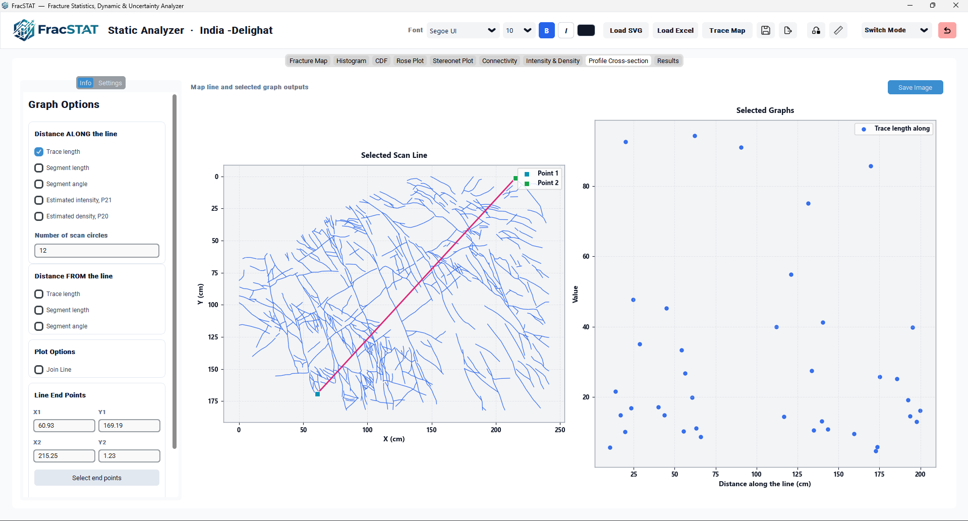
The Profile Cross-section tab is divided into three regions arranged left to right: a tabbed sidebar ("Info" and "Settings" sub-tabs) hosting all analysis and appearance controls, a plot card containing two side-by-side Matplotlib axes — the reference-line map on the left and the derived output plot on the right — and a toolbar above the plot card offering a descriptive label and a Save Image button.
2.1 Left Sidebar — Info Tab
The Info tab is the primary analysis-configuration panel and is organised into four stacked cards:
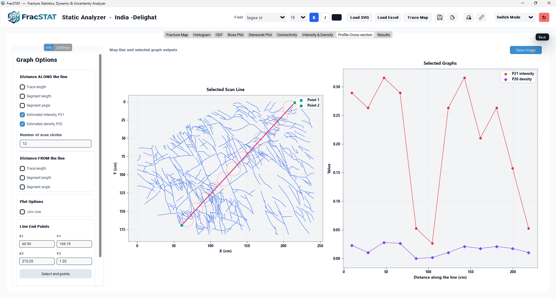
- Distance ALONG the line — five checkboxes selecting which along-line attributes to compute and plot, plus a numeric field controlling the number of circular scan windows used for the intensity/density calculation.
- Distance FROM the line — three checkboxes selecting which perpendicular-offset attributes to compute and plot.
- Plot Options — a single checkbox controlling whether output series are connected by a line.
- Line End Points — four numeric entries (X1, Y1, X2, Y2) defining the reference line, an interactive "Select end points" button for on-map digitizing, and a live status label.
An Update Graphs button at the foot of the Info tab forces an immediate redraw using whatever combination of checkboxes and coordinates is currently set.
2.2 Left Sidebar — Settings Tab
The Settings tab controls the cosmetic appearance of both the map and the output plot: a custom title override, independent legend-position selectors for the map and the output plot, numeric grid- and boundary-line-width fields, a full palette of colour pickers (outer/plot background, grid, plot boundary, scan-line colour, trace colour), a grid-visibility checkbox, and a dedicated Background Image sub-section for overlaying a calibrated real-world photograph beneath the fracture traces. A Reset Defaults button restores every appearance setting in this tab to its factory value.
2.3 Plot Card
The plot card hosts a single Matplotlib Figure containing two subplots created with
add_subplot(121) and add_subplot(122): the left subplot
(graph_map_ax) always shows the fracture-trace network with the current scan line
and, where relevant, the scan-circle windows superimposed; the right subplot
(graph_plot_ax) shows whichever combination of along-line and from-line series the
user has selected, as a scatter plot with optional connecting lines. A toolbar row above the
plot card displays a short descriptive caption and a "Save Image" button that exports the
current figure (including any floating legend) as a high-resolution PNG.
3. Data Input Requirements
The Profile Cross-section module does not import data itself; it consumes the shared
self.results DataFrame that is produced by the Fracture Map tab's loading pipeline
once an SVG trace file or an Excel/CSV orientation/coordinate table has been loaded. The module
requires the following columns to be present with genuine spatial content:
| Column | Description | Required for |
|---|---|---|
X1, Y1, X2, Y2 | Real-world (scaled) segment endpoint coordinates, in the currently selected display unit. | Map rendering; all along-line and from-line calculations. |
Trace | Integer trace (fracture) identifier grouping contiguous segments. | Trace length aggregation for "Trace length along/from". |
Length_m | Per-segment length, always internally expressed in the base unit and re-labelled with the active display unit. | Segment length series; trace length aggregation; intensity/density normalisation. |
StrikeDeg | North-referenced segment strike/azimuth in degrees. | Segment angle along/from series. |
If the currently loaded dataset originates from an orientation-only spreadsheet format (legacy
Strike/Dip fracture-plane tables or Trend/Plunge pole tables) that carries no genuine spatial
coordinates, the module detects this condition — using the same _has_map_geometry
flag consulted by the Fracture Map, Connectivity, and Intensity & Density tabs — and displays
an explanatory empty-state message instructing the user to load an SVG or a spatial Excel/CSV
file with X1, Y1, X2, Y2 columns, rather than attempting a meaningless synthetic-geometry plot.
4. Settings and Controls
4.1 Distance ALONG the Line (Info tab)
| Control | Type | Effect |
|---|---|---|
| Trace length | Checkbox | Plots, for every fracture line-scan intersection, the total length of the parent trace against the along-line distance of that intersection (series label "Trace length along"). |
| Segment length | Checkbox | Plots the length of the individual intersected segment against along-line distance ("Segment length along"). |
| Segment angle | Checkbox | Plots the north-referenced strike of the intersected segment against along-line distance ("Segment angle along"). |
| Estimated intensity, P21 | Checkbox | Enables the Mauldon circular-scanline P21 (fracture length per unit area) series, sampled at evenly spaced windows along the line. |
| Estimated density, P20 | Checkbox | Enables the companion P20 (trace tips per unit area) series from the same scan-window computation. |
| Number of scan circles | Numeric entry | Sets the count of circular sampling windows distributed along the reference line for the P21/P20 calculation; internally clamped to the range 2–200 (default 12). |
4.2 Distance FROM the Line (Info tab)
| Control | Type | Effect |
|---|---|---|
| Trace length | Checkbox | Plots each trace's total length against the perpendicular (signed) distance of that trace's length-weighted midpoint from the reference line ("Trace length from"). |
| Segment length | Checkbox | Plots each segment's length against the perpendicular distance of the segment midpoint from the line ("Segment length from"). |
| Segment angle | Checkbox | Plots each segment's strike against the perpendicular distance of the segment midpoint from the line ("Segment angle from"). |
4.3 Plot Options and Line End Points
| Control | Type | Effect |
|---|---|---|
| Join Line | Checkbox | When enabled, every selected output series is connected with a thin line in addition to its scatter markers, ordered by ascending X value; the two intensity/density series are always joined regardless of this setting, since they represent a continuous sampled function rather than discrete fracture events. |
| X1 / Y1 / X2 / Y2 | Numeric entries | Direct numeric specification of the two reference-line endpoints, in the current display unit. Editing any field and pressing Enter or moving focus away immediately redraws both the map and the derived plot. |
| Select end points | Button | Activates interactive on-map picking mode (see Section 10.1); the next two mouse clicks on the fracture map set Point 1 and Point 2 respectively and populate the four coordinate fields automatically. |
| Status label | Read-only text | Reports the current stage of interactive picking ("Step 1 of 2…", "Step 2 of 2…", or a confirmation once both points are set). |
| Update Graphs | Button | Forces an unconditional redraw of the map and output plot using the current settings; primarily a convenience action, since virtually every other control already triggers a redraw automatically. |
_graphs_convert_units(factor) method multiplies the current X1, Y1, X2, and Y2
values by the appropriate conversion factor and rewrites each StringVar, so the reference line
remains anchored to the same physical location on the map after a unit change rather than
silently keeping its old numeric value in the new unit.
4.4 Settings Tab — Display and Appearance
| Control | Type | Effect |
|---|---|---|
| Custom title (blank = auto) | Text entry | Overrides the automatically generated titles of both the map ("Selected Scan Line") and the output plot ("Selected Graphs") with a single user-supplied string. |
| Map (Legend) Position | Dropdown | Controls placement of the legend on the map subplot; options: best, upper right, upper left, lower left, lower right, center, Outside Right, Outside Bottom. |
| Plot (Legend) Position | Dropdown | Independently controls placement of the legend on the output-plot subplot, using the same option set. |
| Grid line width | Numeric entry | Line width, in points, of the dashed background grid on both subplots (default 0.7). |
| Boundary line width | Numeric entry | Line width of the axis border (spines) on both subplots (default 1.0). |
| Outer background | Colour picker | Fill colour of the Matplotlib Figure canvas outside the plotted axes. |
| Plot background | Colour picker | Fill colour inside both axes (default a light grey, #F3F4F6). |
| Grid colour | Colour picker | Colour of the dashed background grid lines. |
| Boundary colour | Colour picker | Colour of the axis border/spines. |
| Scan line colour | Colour picker | Colour of the reference line drawn on the map (default magenta, #DB2777). |
| Trace colour | Colour picker | Colour of the fracture-trace network drawn on the map (default blue, #2563EB). |
| Show grid lines | Checkbox | Toggles grid visibility on both subplots. |
| Enable custom dimensions | Checkbox | graph_use_custom_size_var, default off. When checked, enables the four Plot Dimensions entry fields below and applies them on the next redraw; when unchecked, the fields are disabled (greyed out) and both subplots instead use Matplotlib's normal automatic subplot layout. |
| Map (W x H) | Numeric entries (px) | Explicit pixel width and height for the map subplot (graph_map_w_var / graph_map_h_var), applied only while "Enable custom dimensions" is checked. Together with the Graph dimensions below, these directly set each subplot's Matplotlib set_position() rectangle (computed from the figure's pixel size), giving pixel‑exact control over subplot size that the default automatic layout cannot offer. |
| Graph (W x H) | Numeric entries (px) | Explicit pixel width and height for the output-plot subplot (graph_plot_w_var / graph_plot_h_var), applied only while "Enable custom dimensions" is checked. |
| Show scale | Checkbox | graph_show_scale_var, default off. Toggles a data‑accurate scale bar in the lower‑right corner of the map subplot — see Section 9.4. |
| Scale colour | Colour picker | graph_color_scale, default #1F2933. Colour used to draw the scale bar (and its label/ticks). |
| Scale style | Dropdown | graph_scale_style_var, default "Solid bar". Chooses how the scale bar is rendered — Solid bar (single filled block), Segmented bar (alternating filled/unfilled quarters), or Ticked line (a plain line with end ticks and no fill). |
| Show real photo behind map | Checkbox | Enables a calibrated background raster image beneath the fracture traces on the map subplot (see Section 10.2). |
| Change Image… | Button | Opens a file-selection dialog to choose or replace the background photograph. |
| Image opacity (0–1) | Numeric entry | Alpha blending value applied to the background photograph. |
| Reset Defaults | Button | Restores every setting in this tab — title, legend positions, widths, all seven colours, the scale-bar toggle/style, the background-image toggle/path/opacity, and the custom plot-dimensions toggle/values — to its factory default via a full reinitialisation of the tab's settings (_init_graph_settings()), then rebuilds the Settings tab UI and redraws. |
5. Mathematical Background
5.1 Reference Line and Parametric Coordinates
The reference (scan) line is defined by its two endpoints P₁ = (x₁, y₁) and P₂ = (x₂, y₂), both expressed in the calibrated real-world display unit. Its Euclidean length is:
A line shorter than 10⁻⁹ display units (i.e. two coincident points) is treated as invalid and suppresses computation, since no meaningful direction can be defined.
5.2 Line–Line Intersection (Distance Along)
For each fracture segment S, with endpoints Q₁ = (x₃, y₃) and Q₂ = (x₄, y₄), the intersection with the reference line is found using the standard two-parameter linear system. Writing the reference line as P₁ + u·(P₂ − P₁) and the segment as Q₁ + v·(Q₂ − Q₁), the intersection parameters (u, v) are obtained from:
where D is the determinant of the direction-vector matrix (the two lines are parallel and non-intersecting whenever |D| < 10⁻¹²). A genuine crossing exists only when both u and v lie within the closed unit interval [0, 1] (subject to a small numerical tolerance of ±10⁻¹⁰ to admit endpoint-touching intersections). The along-line distance of a valid intersection is then:
This is the quantity plotted on the horizontal axis for every "…along" series; it represents how far the intersection point lies from the P₁ end of the reference line, in real-world units.
5.3 Signed Perpendicular Distance (Distance From)
For a point (x, y) — typically a segment or trace midpoint — its signed perpendicular distance from the infinite line through P₁ and P₂ is computed via the two-dimensional cross-product form:
The sign of d_from indicates which side of the reference line the point falls on (consistent with a right-hand rule relative to the line's direction from P₁ to P₂); its magnitude is the shortest Euclidean distance from the point to the line. Because this formula treats the reference line as infinite, contributions may originate from anywhere in the mapped domain, not only from the finite segment between P₁ and P₂ — appropriate for a "from-the-line" transect statistic, where the line represents an axis of reference rather than a bounded sampling window.
5.4 Trace and Segment Midpoints
For the "Segment length/angle from" series, the representative point of each segment is its simple geometric midpoint, ((x₃+x₄)/2, (y₃+y₄)/2). For the "Trace length from" series, each trace is represented by the length-weighted centroid of its constituent segment midpoints:
where xᵢ, yᵢ are the i-th segment's midpoint coordinates and wᵢ is that segment's length (Length_m). If the total weight for a trace is zero or non-finite (e.g. a degenerate zero-length trace), the module falls back to an unweighted arithmetic mean of the segment midpoints.
5.5 Circular Scan-Window Distribution
For the intensity/density series, N circular sampling windows (N = "Number of scan circles") are distributed evenly along the finite reference line. Denoting the user-supplied count as N, the scan-circle radius r and the along-line positions dₖ are:
Each circle is therefore tangent to its neighbours along the line and does not extend past the two line endpoints, which prevents edge circles from being centred outside the mapped area. The circle centre for scan window k is obtained by projecting distance dₖ along the unit direction vector of the reference line.
5.6 Segment–Circle Intersection Count
For each fracture segment and each scan circle of radius r centred at C = (cₓ, c_y), the module must determine (a) whether either endpoint of the segment lies inside the circle, and (b) how many times the segment's finite extent crosses the circle boundary. Writing the segment as A + t·(B − A) for t ∈ [0, 1], substitution into the circle equation ‖A + t(B−A) − C‖² = r² yields the quadratic:
The discriminant Δ = b² − 4ac determines the number of real roots. When Δ ≤ 0 or a ≈ 0 (degenerate segment), the segment does not cross the circle boundary. Otherwise the two roots t₁,₂ = (−b ∓ √Δ)/(2a) are tested against the interval [0, 1]; the number of admissible roots (0, 1, or 2) is the number of true boundary crossings contributed by that segment to that scan circle.
5.7 Fracture Intensity (P21) and Density (P20)
Following the circular-scanline method (Mauldon, 1998; Mauldon et al., 2001; Rohrbaugh et al., 2002), and consistent with the Connectivity and Intensity & Density tabs elsewhere in FracSTAT, each scan circle of radius r accumulates two counts: N_int, the total number of segment–circle boundary crossings (from Section 5.6, counting a fully interior segment once and a partially interior segment once for its single boundary crossing), and m, the number of trace tips that fall strictly inside the circle. The two derived statistics at that scan position are:
A trace's two tips are the start of its first segment and the end of its last segment. Interior polyline vertices — the joins between consecutive segments of the same trace — are deliberately excluded, because they are an artefact of how finely the trace was digitised rather than real fracture terminations.
Trace, ordered by Segment) and tests only those points for
containment. N_int, and hence P21, is unaffected — it is a boundary-crossing count, which is
already invariant to how a trace is subdivided.
P21 has units of [length⁻¹] and estimates the total fracture-trace length per unit sampled area (i.e., areal fracture intensity); P20 has units of [length⁻²] and estimates the number of fracture terminations/nodes per unit sampled area (areal fracture density). Both are evaluated independently at every one of the N scan-window positions along the reference line, producing a one-dimensional profile of intensity/density as a function of position — directly analogous to logging fracture intensity along a physical scanline traverse in the field.
6. Algorithms
6.1 Reference-Line Resolution and Validation
On every redraw, the four coordinate StringVars (X1, Y1, X2, Y2) are parsed as floating-point numbers. If parsing fails for any field, or if the resulting line length is at or below the 10⁻⁹ tolerance, the module renders an explanatory empty-state view ("Enter or select two end points") instead of a plot, preventing a degenerate or undefined geometry from propagating into the downstream calculations.
6.2 Default Line Placement
If none of the four coordinate fields has ever been populated, a default line is generated automatically by taking the minimum and maximum X and Y values across every segment endpoint in the loaded dataset, i.e. the diagonal of the data's axis-aligned bounding box. This guarantees that opening the tab for the first time on a freshly loaded dataset produces an immediately interpretable plot.
6.3 Along-Line Intersection Sweep
The along-line sweep iterates once over every row (segment) of self.results. For
each segment, the parametric line intersection of Section 5.2 is evaluated against the current
reference line. Successful intersections are collected into a list of records containing the
along-line distance, the parent trace's total length (looked up from a pre-computed per-trace
length aggregation), the segment's own length, and the segment's strike; the list is then
sorted by ascending along-line distance before being handed to the plotting stage. This sort
ensures that any optional connecting line (Join Line) traces a coherent path from one end of
the scan line to the other rather than jumping between spatially unrelated points.
6.4 From-Line Aggregation
The perpendicular-distance sweep operates in two independent modes. For trace-level output,
segments are grouped by their Trace identifier (using a pandas groupby), the
length-weighted centroid of each group is computed as in Section 5.4, and the signed distance
of that centroid from the reference line is evaluated once per trace. For segment-level output
(length or angle), the signed distance is evaluated directly at every segment's own midpoint,
without any grouping.
6.5 Circular-Scan Intensity/Density Sweep
This is the most computationally intensive routine in the module. For each of the N scan-circle centres (Section 5.5), every fracture segment in the dataset is tested for endpoint containment (a simple Euclidean-distance-to-centre comparison against the radius) and, where at least one endpoint is outside the circle, for a full segment–circle boundary intersection via the quadratic of Section 5.6. Segments with both endpoints inside the circle contribute no boundary crossing at all (none is possible for a fully interior segment) and are skipped. This is an O(N × M) procedure, where M is the number of fracture segments in the dataset, and is the dominant computational cost of the module for large fracture networks (see Section 11).
The P20 tip count is kept entirely separate from that segment loop. The trace-tip array is built
once, before the sweep, by _graphs_trace_tips(); each scan circle then vectorises a
single distance test over it with np.hypot / np.count_nonzero
(Section 5.7 explains why the tips, and not the segment endpoints, are the correct
population).
def _graphs_intensity_density_along(self, df, line):
    """Utilizes circular scan windows along the line to calculate P21 & P20."""
    centres, radius, distances = self._graphs_scan_circles(line)
    segs = df[["X1", "Y1", "X2", "Y2"]].to_numpy(dtype=float)
    # P20 counts TRACE TIPS, not segment endpoints (Mauldon, Dunne &
    # Rohrbaugh 2001, J. Struct. Geol. 23, 247-258: the circular estimator
    # is P20 = m/(2*pi*r^2) with m the number of trace endpoints inside the
    # window).  Summing int(inside1)+int(inside2) over every SEGMENT counts
    # each interior polyline vertex twice, so a trace digitised into n
    # segments contributed 2n endpoints instead of 2 and P20 scaled with
    # digitisation density rather than with fracture density.
    tips = self._graphs_trace_tips(df)
    intensity, density = [], []

    for cx, cy in centres:
        n_intersections = 0

        for x1, y1, x2, y2 in segs:
            inside1 = math.hypot(x1 - cx, y1 - cy) < radius
            inside2 = math.hypot(x2 - cx, y2 - cy) < radius

            if inside1 and inside2:
                continue
            if inside1 or inside2:
                n_intersections += 1
            else:
                n_intersections += self._graphs_segment_circle_intersections(
                    (x1, y1, x2, y2), (cx, cy), radius)

        if len(tips):
            n_endpoints = int(np.count_nonzero(
                np.hypot(tips[:, 0] - cx, tips[:, 1] - cy) < radius
            ))
        else:
            n_endpoints = 0

        intensity.append(n_intersections / max(4.0 * radius, 1e-12))
        density.append(n_endpoints / max(2.0 * math.pi * radius ** 2, 1e-12))

    return distances, intensity, density


@staticmethod
def _graphs_trace_tips(df):
    """
    The two tips of every trace: start of its first segment and end of its
    last.  Interior polyline vertices are deliberately excluded - they are
    an artefact of digitisation, not fracture terminations.
    """
    if df is None or df.empty or "Trace" not in df.columns:
        return np.empty((0, 2), dtype=float)
    order = ["Trace", "Segment"] if "Segment" in df.columns else ["Trace"]
    ordered = df.sort_values(order)
    pts = []
    for _trace_id, group in ordered.groupby("Trace", sort=False):
        first = group.iloc[0]
        last = group.iloc[-1]
        pts.append((float(first["X1"]), float(first["Y1"])))
        pts.append((float(last["X2"]), float(last["Y2"])))
    return np.asarray(pts, dtype=float) if pts else np.empty((0, 2), dtype=float)
Simplified excerpt of _graphs_intensity_density_along() and its tip helper, showing the per-circle segment–circle crossing count (with the fallback to the algebraic intersection routine for fully exterior segments) and the separate, vectorised trace-tip containment test that feeds P20.
6.6 Interactive Endpoint Picking State Machine
The "Select end points" workflow is implemented as a small state machine attached to
mouse-click events on the map canvas. Activating the button sets an internal picking flag and
clears any previously buffered click, sets the map canvas widget's cursor to
"crosshair" (via configure(cursor="crosshair")) so the user has a
clear visual indicator that picking mode is live, and updates the status label to request the
first click. The first accepted click stores its scene coordinates and draws a temporary,
unfilled "X"‑shaped scatter marker (in the same cyan‑blue, #0891B2, used for the
finalized Point 1 marker — see Section 9.1) plus an adjacent "Point 1" text
label directly onto the map axis, then updates the status label to request the second click.
The second accepted click completes the pair: both points are written into the four coordinate
StringVars, picking mode is deactivated, the cursor is restored, and a full redraw is triggered
automatically — which replaces the temporary "X" marker with the permanent, colour‑coded square
endpoint markers described in Section 9.1. Clicks that land outside the map subplot
(event.inaxes mismatch) or that occur while picking mode is inactive are ignored.
7. Internal Workflow
The end-to-end data flow through the Profile Cross-section module, from user interaction to rendered output, proceeds through the following ordered stages on every redraw request:
- Trigger — a control change (checkbox toggle, Enter/FocusOut on a numeric field, colour selection, map click completing a pair, or the Update Graphs button) invokes the module's central draw routine.
- Axis reset — both the map axis and the output-plot axis are cleared and their background colours re-applied from the current colour-picker state.
- Data availability check — the shared
self.resultstable is inspected; an empty or missing table, or an Excel/CSV source lacking real spatial coordinates, produces an explanatory empty-state message and the workflow halts. - Default-line seeding — if no coordinates have ever been entered, the bounding-box diagonal default line (Section 6.2) is computed and written into the coordinate fields.
- Line resolution — the four coordinate fields are parsed and validated (Section 6.1); failure again halts the workflow with an explanatory message.
- Map rendering — the full fracture-trace network is drawn as a LineCollection, the reference line is drawn on top in the selected scan-line colour, endpoint markers are added, and — if the intensity/density checkboxes are active — every scan-circle outline is drawn faintly for visual reference. The optional calibrated background photograph is drawn beneath all vector content.
- Output collection — each enabled checkbox invokes its corresponding computation routine (Sections 6.3–6.5); results are assembled into a list of (label, x-values, y-values, colour, marker) tuples.
- Output rendering — each collected series is scatter-plotted on the output axis in its assigned colour and marker shape; the intensity/density series are always also line-connected (since they represent a continuous function), while other series are connected only if Join Line is enabled — in which case points are first sorted by X to guarantee a directionally coherent line.
- Cosmetic finishing — titles (custom or automatic), axis labels using the active display unit, legends at their configured positions, grid lines, and axis-spine styling are applied to both subplots.
- Canvas draw — both subplots are redrawn to the screen via the Matplotlib TkAgg canvas's
draw_idle()call, and the parent Figure'stight_layout()is invoked to avoid label clipping.
8. Statistical Methods and Quantitative Outputs
Unlike several other Static Analyzer tabs (Histogram, CDF, Rose Plot), the Profile Cross-section module does not fit theoretical statistical distributions; its statistical content is instead the raw sampled series described in Section 5, together with the derived P21/P20 areal estimators. The following table summarises every output series that can appear on the right-hand plot, together with its physical units and the geological question it is designed to answer.
| Series | Horizontal axis | Vertical axis / units | Geological question addressed |
|---|---|---|---|
| Trace length along | Distance along line | Trace length (display unit) | Do longer fractures cluster at particular positions along the transect (e.g. near a fault core)? |
| Segment length along | Distance along line | Segment length (display unit) | Is local fracture length variable at fine spatial resolution along the transect? |
| Segment angle along | Distance along line | Strike (degrees) | Does fracture orientation rotate systematically along the transect (e.g. across a fold hinge)? |
| P21 intensity | Distance along line | Fracture length per unit area (unit⁻¹) | How does areal fracture intensity vary spatially, independent of network orientation bias? |
| P20 density | Distance along line | Trace tips per unit area (unit⁻²) | How does the areal density of fracture terminations vary spatially? |
| Trace length from | Perpendicular distance from line | Trace length (display unit) | Are longer fractures preferentially located on one side of a chosen reference feature (e.g. a bedding plane or fault)? |
| Segment length from | Perpendicular distance from line | Segment length (display unit) | Is segment length asymmetric about the reference line? |
| Segment angle from | Perpendicular distance from line | Strike (degrees) | Does fracture orientation differ systematically on either side of the reference line? |
All along-line and from-line series are discrete point clouds, one point per fracture segment (or per trace, for the trace-length variants); the P21/P20 series are, by contrast, smooth sampled functions of position with exactly N points each, where N is the user-specified scan-circle count.
9. Visualization Components
9.1 Reference-Line Map (Left Subplot)
The map subplot renders the complete fracture-trace network as a LineCollection in the user-selected trace colour, the reference line as a bold coloured segment in the scan-line colour, and square markers at Point 1 (cyan-blue, #0891B2) and Point 2 (green, #16A34A) labelled accordingly in the legend. When either intensity or density is enabled, every scan-circle boundary is drawn as a thin, low-opacity red outline so the user can visually confirm the spatial extent each sample window covers relative to the fracture network. Axis limits are padded by five percent of the data range on each side (with a minimum one-unit pad) so traces are never clipped at the figure edge, and the aspect ratio is fixed to "equal" so that geometric distances and angles are not visually distorted. An optional scale bar can also be drawn in the lower-right corner of this subplot — see Section 9.4.
9.2 Output Plot (Right Subplot)
The output subplot is a Cartesian scatter plot with an optional connecting line per series, using Matplotlib's automatic colour-differentiated markers (circle, square, triangle, and diamond markers are assigned per series in the implementation) so that multiple simultaneously enabled series remain visually distinguishable. The horizontal axis is always labelled "Distance along/from line (unit)"; the vertical axis is deliberately left as a generic "Value" label, since the module may display several physically distinct quantities (length in display units; angle in degrees; intensity in unit⁻¹; density in unit⁻²) simultaneously on a shared axis — the legend, not the axis label, is the authoritative key to each series' physical meaning in that situation.
9.3 Legends and Titles
The map and output-plot legends are positioned independently via their respective dropdown
controls. "Outside Right" places the legend just beyond the right edge of the axis using a
bbox_to_anchor offset; "Outside Bottom" places it below the axis in a multi-column
row. Both subplots' titles default to descriptive automatic text ("Selected Scan Line" and
"Selected Graphs" respectively) but are overridden together by the single Custom Title field
when non-empty.
9.4 Scale Bar (_add_graphs_scale_bar)
When "Show scale" is enabled, _add_graphs_scale_bar() adds a data‑accurate
mpl_toolkits.axes_grid1.anchored_artists.AnchoredSizeBar anchored to the
lower‑right corner of the map subplot (loc="lower right"). The bar's physical
length is chosen by a "nice number" heuristic — the largest value of the form
1, 2, or 5 × 10ⁿ that does not exceed 22% of the map's current X‑axis span — so the
labelled length is always a round, easily read figure rather than an arbitrary fraction of the
map width. If the project's display unit is metres and the computed length is 1000 or
greater, the label is shown in kilometres (e.g. "2 km") instead of an unwieldy metre value; for
any other unit, or a length under 1000 m, the label uses the display unit unchanged. The
three "Scale style" options are all drawn from the same underlying bar: Solid bar
leaves the default filled rectangle as‑is; Segmented bar hides that rectangle and
rebuilds it as four alternating filled/unfilled quarter‑segments in the chosen scale colour
and the Plot background colour; Ticked line suppresses the vertical bar height
entirely, leaving only the horizontal line and its end ticks.
10. Advanced and Interactive Features
10.1 Interactive On-Map Line Digitizing
Rather than requiring manual coordinate entry, the user may click the "Select end points" button and then click twice directly on the fracture map to define the reference line visually. The first click is rendered immediately as a temporary "X"-shaped marker labelled "Point 1" (see Section 6.6) so the user receives instant visual confirmation; the second click completes the line, writes both coordinate pairs into the numeric entry fields (so they remain editable afterward), and triggers a full recalculation that redraws both endpoints as the permanent square markers described in Section 9.1. This workflow is particularly useful for aligning the reference line with a specific geological feature visible on a loaded background photograph (see Section 10.2), such as a fault trace or bedding contact, without needing to first read off its coordinates.
10.2 Calibrated Background Photograph Overlay
The Settings tab's Background Image sub-section allows a real-world photograph — typically the same calibrated image used to establish the map's pixel-to-real-world scale via the Scale Calibration tool — to be displayed beneath the fracture-trace network and reference line. The module automatically searches for a suitable image in the following priority order: a path explicitly already stored for this tab, the Fracture Map tab's own calibrated background image path, the Trace Map tool's saved sidecar PNG file (co-located with the source SVG), and whichever background image has already been shared to the Dynamic Analyzer workspace via the launcher's cross-workspace shared state. This means a background image only ever needs to be uploaded once, in any single workspace, for it to become available in the Profile Cross-section map as well.
The overlay respects the same real-world bounding-box extent as the fracture network and is
drawn with origin="upper" and an explicit extent mapping so that image row order
correctly matches the (frequently inverted) Y-axis convention used by SVG-derived fracture
maps. Opacity is independently adjustable via the Image opacity field, allowing the fracture
traces to remain legible against a bright or high-contrast photograph.
10.3 Move Elements / Free Layout Mode
Like every other plot-bearing tab in the Static Analyzer, the Profile Cross-section map and plot participate in the workspace-wide "Move Elements" editing mode (toggled from the shared header toolbar). When active, individual Matplotlib axes on the canvas may be freely repositioned by click-and-drag, which is useful when preparing a combined figure for external publication or reporting, since the relative sizing of the map versus the output plot can be adjusted without leaving the application.
10.4 Save Image Export
The Save Image button exports the full two-panel Figure — map and output plot together, with
legends, titles, and any manual layout adjustments included — as a PNG raster at the
application-wide configured export resolution (Settings page "Plot export DPI", default
300 dpi). The exported filename is automatically constructed from the current project
name, a fixed "static_graphs" tag, and a timestamp, and is written into the project's
FracSTAT_plot_exports subfolder.
11. Performance Optimization
The along-line intersection sweep (Section 6.3) and the from-line aggregation (Section 6.4) are both O(M) in the number of fracture segments M, since each segment is tested against a single fixed reference line exactly once; these therefore scale comfortably even for networks containing many thousands of segments.
The circular-scan intensity/density sweep (Section 6.5) is inherently O(N × M), because every one of the N scan circles must be tested against every one of the M segments independently — there is no shared geometric pre-filtering between different circles in the current implementation. Because N (the scan-circle count) is user-controlled and bounded by the interface to at most 200, and because this calculation is only performed at all when the intensity or density checkboxes are actively enabled, the practical cost is kept manageable: with a typical N of 12 and networks of a few thousand segments, the calculation completes essentially instantaneously; very large fracture datasets combined with a high scan-circle count will scale linearly in both factors, and the user is advised to reduce the scan-circle count if redraw responsiveness becomes noticeable on very dense datasets.
All heavy geometric loops in this module are implemented at the Python level (rather than being vectorised with NumPy), unlike the analogous circular-scanline computation in the Intensity & Density tab, which is fully vectorised for its grid-based Mauldon calculation. Consequently, the Profile Cross-section module's intensity/density feature is best used as a targeted, along-transect diagnostic rather than as a replacement for the grid-based global P21/P20 mapping already provided by the dedicated Intensity & Density tab.
12. Practical Examples
12.1 Worked Example — Along-Line Intensity Profile Across a Fault Damage Zone
Scenario: a fracture-trace SVG has been digitized from an outcrop photograph spanning a mapped fault trace, with the fault oriented roughly northeast–southwest across the centre of the image.
- Load the SVG file via the workspace header's Load SVG button, and confirm the profile scale using the Scale tool so that real-world distances are correctly calibrated.
- Open the Profile Cross-section tab. A default diagonal reference line appears automatically across the full mapped extent.
- In the Info tab, click "Select end points", then click once at the outcrop edge on one side of the fault and once on the opposite edge, so that the new reference line crosses the fault trace roughly perpendicular to its strike.
- Enable "Estimated intensity, P21" and set "Number of scan circles" to a value such as 20 for finer spatial resolution along the transect.
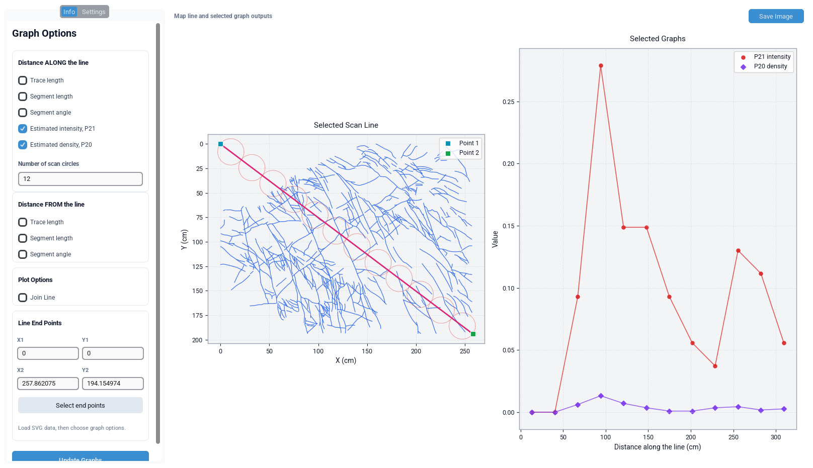
- Inspect the resulting P21 profile in the output plot: a pronounced local maximum in P21 near the along-line position corresponding to the fault trace is diagnostic of a fracture damage zone, and the profile's decay away from that position can be used to estimate the damage-zone half-width.
- Optionally enable "Segment angle along" simultaneously to check whether fracture orientation also changes systematically within the damage zone (e.g. rotation toward parallelism with the fault as the fault core is approached).
12.2 Worked Example — Bedding-Perpendicular Asymmetry Check
Scenario: the user suspects that fracture length differs systematically above versus below a particular bedding contact visible in the mapped image.
- Set the reference line to run exactly along the bedding contact, either by typing its two endpoint coordinates directly or by clicking along it on a calibrated background photograph.
- Enable "Trace length from" in the Distance FROM the line card.
- Read the resulting scatter plot: points with positive perpendicular distance lie on one side of the contact, points with negative distance on the other; a visible asymmetry in the spread or central tendency of trace length between the positive and negative halves of the plot supports a genuine lithological or mechanical-stratigraphic control on fracture length.
13. Geological Interpretation
The Profile Cross-section module reproduces, in digital form, the classical field scanline survey that underpins much of quantitative structural-geology fracture characterisation. Its outputs support several standard interpretive workflows:
- Damage-zone characterisation — a local increase in P21/P20 intensity and/or a systematic rotation of fracture strike toward the along-line position of a mapped fault is the standard diagnostic signature of a fault damage zone (Faulkner et al., 2010), and the half-width of the elevated-intensity interval provides a first-order estimate of damage-zone width for comparison with regional fault-scaling relationships (Savage and Brodsky, 2011).
- Stratigraphic (bed-thickness) control on fracture length — fracture length and spacing are frequently observed to correlate with mechanical layer thickness in layered sedimentary sequences (Ladeira and Price, 1981; Narr and Suppe, 1991; Bai and Pollard, 2000). Running the reference line parallel to bedding and inspecting the "Segment/Trace length from" plots on either side of a bed boundary can reveal whether fracture populations terminate systematically at that boundary, consistent with bed-confined ("layer-bound") fracturing.
- Anisotropy-independent intensity estimation — because straight-scanline (P10) sampling is well known to be biased against fracture sets sub-parallel to the scanline (Terzaghi, 1965), the circular-window P21/P20 estimator implemented here removes this orientation bias (Mauldon et al., 2001; Rohrbaugh et al., 2002), making the reported intensity/density profile more representative of the true areal fracture population than a simple count of scanline crossings would be.
- Spatial-trend screening — because the reference line can be placed anywhere and reoriented freely, the module functions as a rapid, exploratory tool for screening a mapped area for spatial trends in any measured fracture attribute before committing to a more elaborate grid-based analysis in the dedicated Intensity & Density tab.
14. Implementation Notes
The module is implemented as the StaticGraphsTab Python mixin class, combined
into StaticAnalyzerApp via multiple inheritance together with the other Static
Analyzer tab mixins. All interactive controls are built with ui_common.qtk (PySide6) widgets
(CTkCheckBox, CTkEntry, CTkOptionMenu,
CTkButton) bound directly to Tk-style Variable objects, so that reading a
control's current value anywhere in the drawing routine is simply a matter of calling
.get() on the corresponding variable; every control that should trigger a redraw
is wired either to its variable-change command callback or to a bound
Return/FocusOut keyboard event.
Colour selections are handled by a shared _StaticColorButton widget (used
identically across all Static Analyzer tabs) that opens a small swatch-and-hex-entry dialog and
invokes a callback with the chosen hex string; this callback both updates the corresponding
Python attribute and immediately triggers a redraw, so colour changes are reflected live
without a separate "Apply" step.
The module maintains no persistent computed-result cache between redraws; because both the
along/from sweeps and the circular-scan sweep are computed freshly from
self.results on every redraw, the displayed output is always guaranteed to be
consistent with whatever fracture dataset and profile-scale calibration are currently active
elsewhere in the Static Analyzer, at the cost of recomputation on every appearance-only change
(mitigated, as noted in Section 11, by the low cost of the along/from sweeps).
Background-image loading is itself cached at the instance level (a simple path-keyed cache holding the most recently loaded and decoded image array), so that repeated redraws while only a cosmetic setting (such as opacity) changes do not repeatedly re-read and re-decode the same image file from disk.
15. Limitations
| Limitation | Description |
|---|---|
| Unvectorised circular-scan loop | The circular-scan intensity/density computation is an unvectorised, per-segment Python loop and therefore does not scale as efficiently as the equivalent grid-based Mauldon calculation in the dedicated Intensity & Density tab; very large datasets combined with a high scan-circle count may notice a perceptible delay. |
| Infinite-line "distance from" | The "distance from" calculation treats the reference line as infinite in both directions, so points far outside the finite segment between the two chosen endpoints still contribute a perpendicular-distance value; this is by design (consistent with treating the line as an axis of reference) but should not be mistaken for a bounded corridor sample. |
| Planar assumption | The module assumes a two-dimensional, effectively planar fracture-trace map; no correction is applied for outcrop-surface curvature, oblique viewing angle, or true 3-D fracture orientation beyond what is already encoded in the loaded strike values. In particular no Terzaghi orientation-bias weighting is applied to the along-line crossing counts (Terzaghi, 1965); the circular-window P21/P20 series is the orientation-robust estimator on this page. |
| Topological terminology follows the trace-map convention | Counted trace tips are the isolated ends of digitised traces, which correspond to I-nodes in fracture-network topology; abutting (Y) and crossing (X) nodes are not classified here, and the terms are used as defined in the fracture-network glossary (Peacock et al., 2016). Topological connectivity is the Connectivity tab's remit (Sanderson and Nixon, 2015). |
16. References
Sources are listed alphabetically within each group. In-text citations throughout this page link to the corresponding entry below.
16.1 Fracture Intensity and Circular-Window Sampling
- Dershowitz, W. S., & Herda, H. H. (1992). Interpretation of fracture spacing and intensity. In Proceedings of the 33rd U.S. Symposium on Rock Mechanics (pp. 757–766). Balkema, Rotterdam. ISBN 978-90-5410-045-3. (Source of the Pij notation used for P10, P20 and P21.)
- Mauldon, M. (1998). Estimating mean fracture trace length and density from observations in convex windows. Rock Mechanics and Rock Engineering, 31(4), 201–216. https://doi.org/10.1007/s006030050021
- Mauldon, M., Dunne, W. M., & Rohrbaugh, M. B. (2001). Circular scanlines and circular windows: new tools for characterizing the geometry of fracture traces. Journal of Structural Geology, 23(2–3), 247–258. https://doi.org/10.1016/S0191-8141(00)00094-8 (P21 = N/(4r), P20 = m/(2πr²) with m the count of trace endpoints.)
- Rohrbaugh, M. B., Dunne, W. M., & Mauldon, M. (2002). Estimating fracture trace intensity, density, and mean length using circular scan lines and windows. AAPG Bulletin, 86(12), 2089–2104. https://doi.org/10.1306/61EEDE0E-173E-11D7-8645000102C1865D
16.2 Sampling Bias and Survey Practice
- Priest, S. D. (1993). Discontinuity Analysis for Rock Engineering. Chapman & Hall, London. https://doi.org/10.1007/978-94-011-1498-1 (Scanline survey practice and one-dimensional spacing statistics.)
- Terzaghi, R. D. (1965). Sources of error in joint surveys. Géotechnique, 15(3), 287–304. https://doi.org/10.1680/geot.1965.15.3.287 (Orientation bias of linear sampling.)
- Watkins, H., Bond, C. E., Healy, D., & Butler, R. W. H. (2015). Appraisal of fracture sampling methods and a new workflow to characterise heterogeneous fracture networks at outcrop. Journal of Structural Geology, 72, 67–82. https://doi.org/10.1016/j.jsg.2015.02.001
- Zeeb, C., Gomez-Rivas, E., Bons, P. D., & Blum, P. (2013). Evaluation of sampling methods for fracture network characterization using outcrops. AAPG Bulletin, 97(9), 1545–1566. https://doi.org/10.1306/02131312042
16.3 Fracture-Network Structure and Geological Controls
- Bai, T., & Pollard, D. D. (2000). Fracture spacing in layered rocks: a new explanation based on the stress transition. Journal of Structural Geology, 22(1), 43–57. https://doi.org/10.1016/S0191-8141(99)00137-6
- Faulkner, D. R., Jackson, C. A. L., Lunn, R. J., Schlische, R. W., Shipton, Z. K., Wibberley, C. A. J., & Withjack, M. O. (2010). A review of recent developments concerning the structure, mechanics and fluid flow properties of fault zones. Journal of Structural Geology, 32(11), 1557–1575. https://doi.org/10.1016/j.jsg.2010.06.009
- Ladeira, F. L., & Price, N. J. (1981). Relationship between fracture spacing and bed thickness. Journal of Structural Geology, 3(2), 179–183. https://doi.org/10.1016/0191-8141(81)90013-4
- Narr, W., & Suppe, J. (1991). Joint spacing in sedimentary rocks. Journal of Structural Geology, 13(9), 1037–1048. https://doi.org/10.1016/0191-8141(91)90055-N
- Peacock, D. C. P., Nixon, C. W., Rotevatn, A., Sanderson, D. J., & Zuluaga, L. F. (2016). Glossary of fault and other fracture networks. Journal of Structural Geology, 92, 12–29. https://doi.org/10.1016/j.jsg.2016.09.008
- Sanderson, D. J., & Nixon, C. W. (2015). The use of topology in fracture network characterization. Journal of Structural Geology, 72, 55–66. https://doi.org/10.1016/j.jsg.2015.01.005
- Savage, H. M., & Brodsky, E. E. (2011). Collateral damage: Evolution with displacement of fracture distribution and secondary fault strands in fault damage zones. Journal of Geophysical Research: Solid Earth, 116, B03405. https://doi.org/10.1029/2010JB007665
Methods statement for the Profile Cross-section tab. If a figure produced by this tab appears in a publication, the details below are what a reader needs in order to reproduce it, and are what the citations above assume:
Fracture attributes were sampled along a two-point reference line placed on a digitised trace map, reproducing a scanline traverse (Priest, 1993). Along-line intensity and density were estimated with N non-overlapping circular windows of radius r = L/(2N) centred on the line, using P21 = Nint/(4r) and P20 = m/(2πr²), where Nint is the count of segment–boundary crossings and m the count of trace tips inside the window (Mauldon, 1998; Mauldon et al., 2001; Rohrbaugh et al., 2002); the Pij notation follows Dershowitz and Herda (1992). Because circular windows are orientation-unbiased, no Terzaghi weighting was applied (Terzaghi, 1965). Reported values are two-dimensional trace-map estimates and remain subject to truncation and censoring bias (Zeeb et al., 2013; Watkins et al., 2015). Node and network terminology follows Peacock et al. (2016); topological connectivity is reported by the Connectivity tab (Sanderson and Nixon, 2015). Interpretations of along-profile intensity peaks as damage zones, or of length–thickness relationships as stratigraphic control, should cite the relevant structural literature (Faulkner et al., 2010; Savage and Brodsky, 2011; Ladeira and Price, 1981; Narr and Suppe, 1991; Bai and Pollard, 2000). State the reference-line endpoints, the display unit, and the scan-circle count N alongside any published profile, since r and hence both estimators depend on N.