Uncertainty LHS Tab
The Latin Hypercube Sampling (LHS) tab is part of FracSTAT's Uncertainty Analyzer, a self-contained probabilistic workspace for evaluating fault and fracture stability under uncertain stress, pore-pressure, rock-strength, and orientation conditions. Unlike a deterministic calculation that returns one value for each input condition, the LHS workflow propagates uncertainty through the Mohr–Coulomb fault-stability calculation and produces probability distributions for Slip Tendency (Ts), Dilation Tendency (Td), Fracture Susceptibility (Sf), and Coulomb Failure Index (Fsi).
uncertainty_lhs_tab.py. It creates the shared sampling workspace from
uncertainty_sampling_tab.py with the sampling method fixed to "lhs".
The LHS and Monte Carlo tabs therefore share the same controls, analysis modules, plots, caching,
validation and export infrastructure; the principal difference is how the underlying sample
coordinates are generated.
On this page
- 1. Purpose and scope
- 2. Interface overview
- 3. Data input
- 4. Settings and controls
- 5. Mathematical background
- 6. Algorithms
- 7. Internal workflow
- 8. Statistical methods and validation
- 9. Visualization
- 10. Advanced features
- 11. Performance optimization
- 12. Practical examples
- 13. Geological interpretation
- 14. Implementation notes
- 15. Limitations
- 16. References
1. Purpose and Scope
The LHS module provides a stratified, variance-reduced probabilistic simulation environment for evaluating mechanical stability of faults and fractures. It propagates uncertainty in the three principal stresses, pore pressure, cohesion, friction, SHmax azimuth, strike and dip through the same Mohr–Coulomb mechanics used by the deterministic stability calculator.
The Uncertainty Analyzer is independent of the Static and Dynamic Analyzer workspaces. Its input tables, sampling settings, cached results and session state are private to the uncertainty workspace and are not written back into the Static/Dynamic shared project cache.
1.1 What the LHS module provides
- Stratified Latin Hypercube sampling with reproducible random seeds.
- Uncertain stress, strength, pressure and orientation inputs.
- Mohr–Coulomb fault-stability calculations for every realization.
- Probability distributions for Ts, Td, Sf and Fsi.
- Descriptive statistics, convergence diagnostics and analytical/reference validation.
- SRC and PRCC sensitivity analysis.
- Spatial probability mapping when coordinate data are supplied.
- Publication-oriented visualization, image export and tabular result export.
2. Interface Overview
The LHS tab occupies one page of the CTkTabview created by
UncertaintyAnalyzerApp._build_workspace_tabs. It contains the same workspace
structure as the Monte Carlo tab, but uses sampling_method="lhs".
2.1 Workspace header
The shared header provides Load Excel/CSV, mode switching between Dynamic and Static workspaces, and a live status bar. The status area reports loading results, simulation outcomes, convergence state, cancellation and export locations. SVG loading and scale calibration are disabled in this workspace because the uncertainty module works with tabular fault data rather than digitized fracture traces.
2.2 Nested analysis modules
Each sampling tab contains six nested modules in a fixed order: Geomechanics, Statistics, Sensitivity, Visualization, Spatial Probability Map, and Validation & Export. Only the currently visible module is redrawn after a run or fault switch, which keeps large ensembles responsive.
2.3 Shared control bar
| Control | Function |
|---|---|
| SAMPLES | Requested LHS design size N per fault. Valid range: 10–100,000. |
| SEED | Integer seed forwarded to scipy.stats.qmc.LatinHypercube for reproducible designs. |
| FAULT | Selects All Faults for a population run or one specific loaded fault. |
| Run Latin Hypercube Sampling | Starts the background simulation using the current settings. |
| Cancel | Requests cooperative cancellation of an active simulation. |
| Method badge | Displays Latin Hypercube Sampling. |
| Source badge | Displays the loaded input filename and worksheet when applicable. |
3. Data Input
3.1 Loading fault/fracture orientation data
Use Load Excel/CSV in the shared header. Workbook loading is performed on a background thread so the Qt interface remains responsive. Multi-sheet workbooks open a worksheet selection dialog; CSV files and single-sheet workbooks proceed directly.
Column recognition is alias-driven. FracSTAT normalizes header names to lower-case, alphanumeric-only text and maps recognized aliases to canonical fields.
| Canonical field | Recognized header aliases |
|---|---|
| fault_id | ID No, ID, Frac_ID, Fault_ID, Fracture_ID, Fault Name, Fault_Name |
| strike | Strike |
| dip | Dip |
| sigma1 / sigma2 / sigma3 | Sigma 1 / Sigma 2 / Sigma 3, including underscore/no-space variants |
| friction | Friction Coefficient, Friction, mu |
| cohesion | Cohesion, C0, C, Cohesive Strength |
| pore_pressure | Pore Pressure, Pf |
| shmax | SHmax, S Haz, Shaz, Maximum Horizontal Stress Azimuth |
3.2 Input validation
| Rule | Enforcement |
|---|---|
| Strike and Dip numeric | Missing or non-numeric values raise an error before the fault is added. |
| Strike range | 0° ≤ Strike < 360°. Strike = 360° is rejected. |
| Dip range | 0° ≤ Dip ≤ 90°. |
| Fault ID uniqueness | Duplicate identifiers are rejected. |
| Fault ID non-empty | Blank or whitespace-only identifiers are rejected. |
| No input file | A synthetic “Representative plane” with Strike 45° and Dip 60° is used. |
3.3 Spatial coordinate files
The Spatial Probability Map has a separate coordinate-loading path. Two coordinate layouts are recognized automatically.
| Layout | Required columns | Optional columns | Rendering |
|---|---|---|---|
| Point coordinates | ID, X, Y | Easting/Northing and unit-tagged headers | One coloured marker per fault |
| Trace coordinates | X1, Y1, X2, Y2 | ID | One coloured line segment per fault |
Units can be detected from bracketed or parenthesized headers such as X-Coordinate [m]
or X [km]. Input and display units can be independently selected from km, m, cm and mm.
4. Settings and Controls
4.1 Geomechanics — uncertainty inputs
| Section | Inputs | Distribution choices | Notes |
|---|---|---|---|
| Principal stresses | σ1, σ2, σ3 (MPa) | Normal, Truncated Normal, Gaussian, Lognormal, Gamma | σ1 > σ2 > σ3 and SD(σ1) ≥ SD(σ2) ≥ SD(σ3). |
| Rock strength & pressure | Friction, Cohesion, Pore Pressure | Same choices, plus Beta for friction | Friction is bounded [0,1]; cohesion and pore pressure are non-negative. |
| Fault & stress orientation | Strike, Dip, SHmax (deg) | Von Mises or Fisher 3D | Each orientation row has concentration parameter k; Fisher 3D couples Strike and Dip. |
4.1.1 Per-row controls
| Control | Description |
|---|---|
| Mean | Central value in physical units. Per-fault values from the loaded file can override the global mean. |
| STDV / k | Standard deviation for stress/strength rows; concentration k for orientation rows. Higher k means tighter orientation clustering. |
| Distribution | Selects the probability law used for the input. |
| Min / Max | Available for Uniform or Beta. Blank values allow automatic bound derivation from mean/SD. |
| Auto STDV | Sets all STDV fields in a section to a selected 1–50% of the current mean. |
4.1.2 Stress regime selector
The stress-regime selector provides Normal Faulting (Sv = σ1), Strike-Slip (Sv = σ2), and Reverse/Thrust (Sv = σ3). The selected regime controls which sampled principal stress is mapped to the vertical slot used by the stability calculation. The displayed σ1 > σ2 > σ3 ordering remains unchanged.
4.1.3 Effective-stress switch
Use effective principal stresses controls whether pore pressure is subtracted from the stress terms used by Ts, Td and Fsi. Changing the switch recalculates the active and cached metrics without re-running the sampler. Sf is not affected by it: a sustainable pore-pressure increase only exists under the effective-stress principle, so Sf — and the failure flag derived from it — is always computed on σ′n = σn − Pp (Section 5.5).
4.1.4 Plot appearance
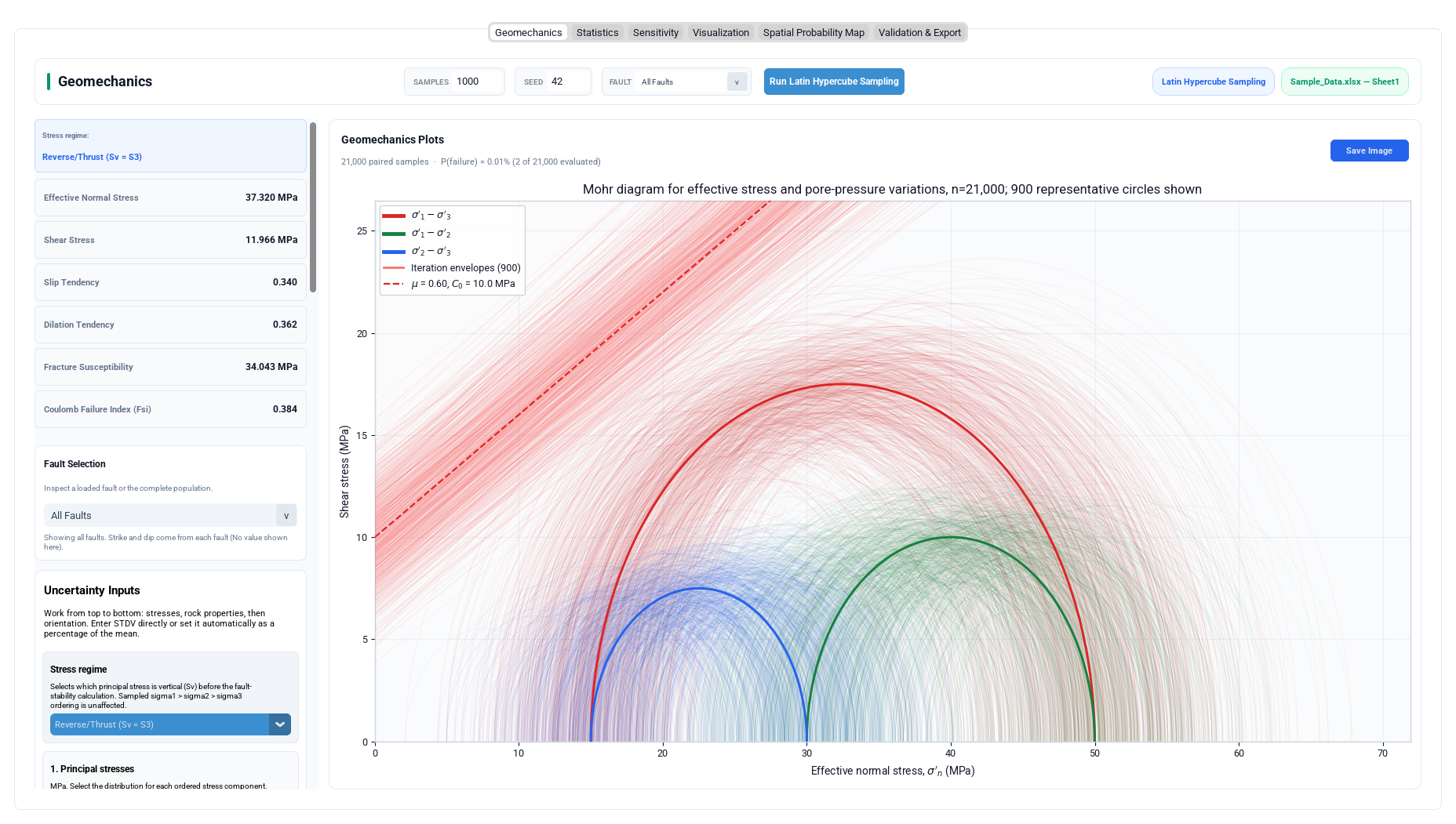
Geomechanics appearance controls include Mohr uncertainty diagrams, total-stress Mohr circles, stress-scatter styling, backgrounds, grid, colour scales, failed-point highlighting, Coulomb envelope and Mohr-circle visibility, legends, axis scale and explicit plot width/height in pixels.
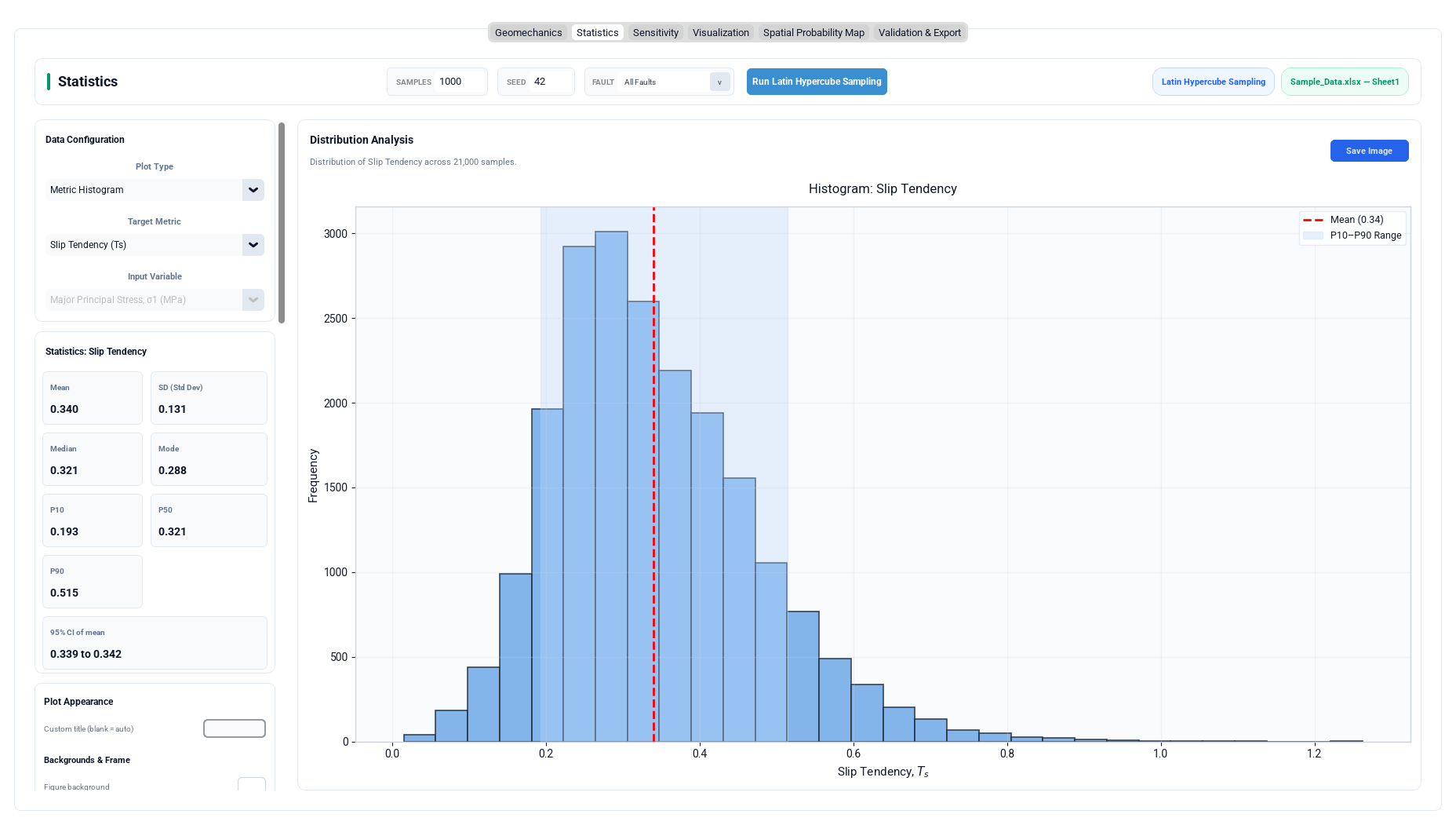
4.2 Statistics module
| Control | Purpose |
|---|---|
| Plot Type | Metric Histogram, Sampled Input Distribution, Input-Response Plot, or Probabilistic Response (Single). |
| Target Metric | Ts, Td, Sf or Fsi. |
| Input Variable | One of the nine sampled inputs for input-dependent plots. |
| Descriptive statistics | Mean, SD, Median, Mode, P10, P50, P90 and 95% CI of the mean. |
| Appearance | Background/grid, bins, alpha/hatch, scatter styling, mean/range styling, trend curve, axes, legend and plot size. |
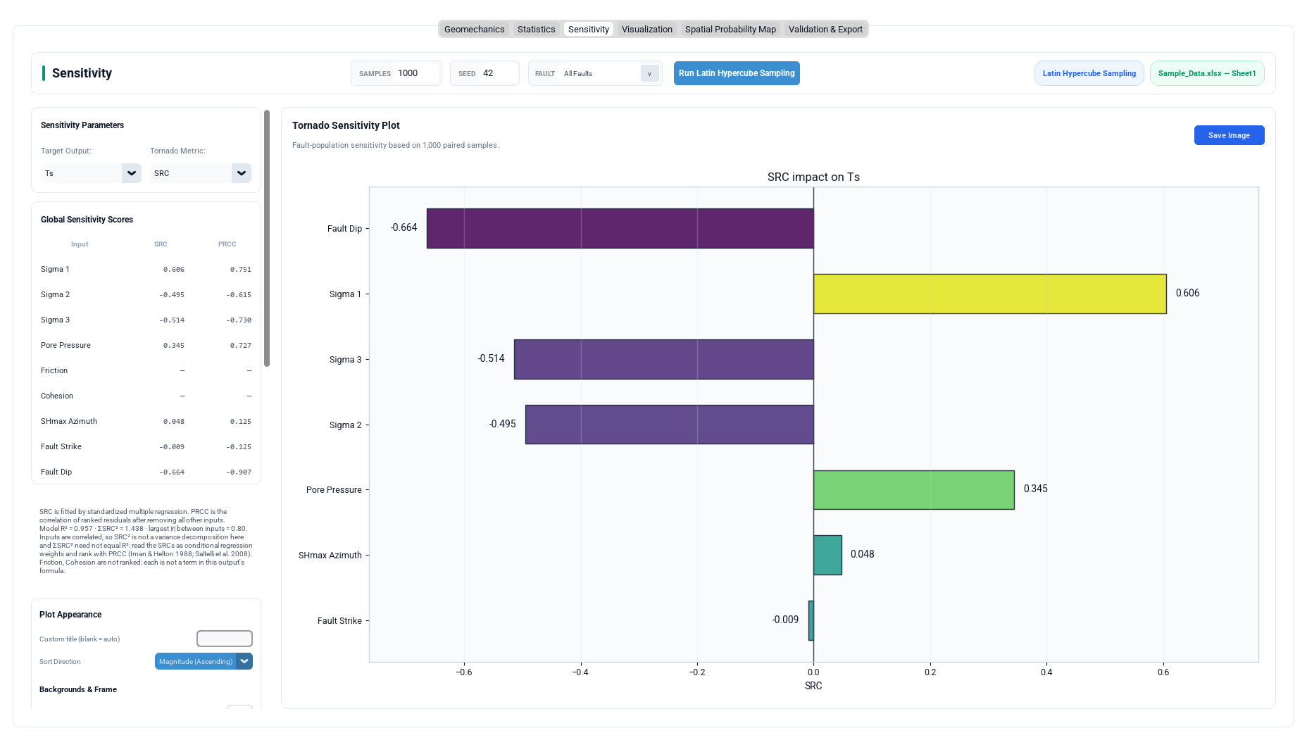
4.3 Sensitivity module
| Control | Purpose |
|---|---|
| Target Output | Selects Ts, Td, Sf or Fsi. |
| Tornado Metric | Switches between SRC and PRCC. |
| Global Sensitivity Scores | Reports SRC/PRCC for all nine inputs. |
| Sort Direction | Magnitude ascending, descending, or declaration order. |
| Bar styling | Height, alpha, edge styling, colour mode and colour scale. |
| Value labels | Displays numeric values on the bars. |
4.4 Validation & Export
| Control | Function |
|---|---|
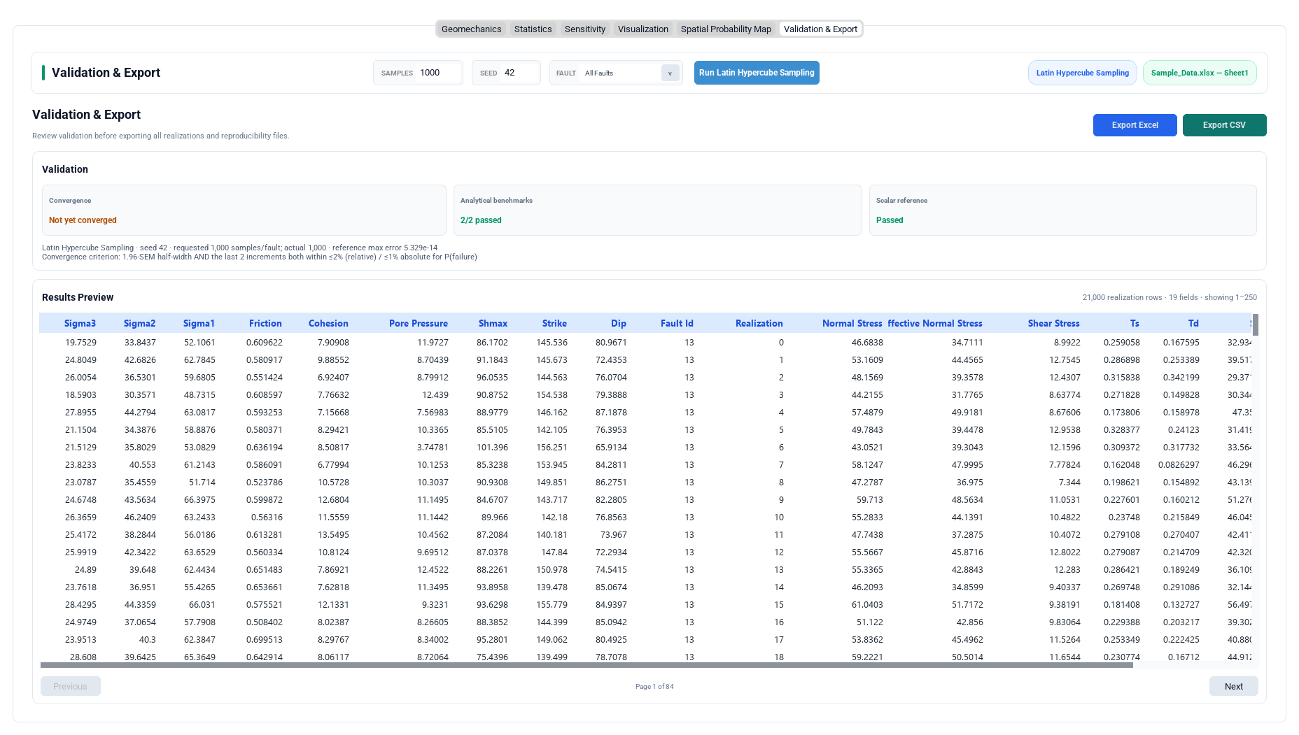
| Convergence / Benchmarks / Reference cards | Pass/fail summaries for the three validation checks. |
| Results Preview | Paginated read-only view of realization and calculated columns, 250 rows per page. |
| Export Excel | Writes Results, Convergence, Benchmarks, Reference Check and Metadata worksheets to one .xlsx workbook. |
| Export CSV | Writes results.csv, convergence.csv, analytical_benchmarks.csv and metadata.json. |
4.5 Spatial Probability Map
| Control | Purpose |
|---|---|
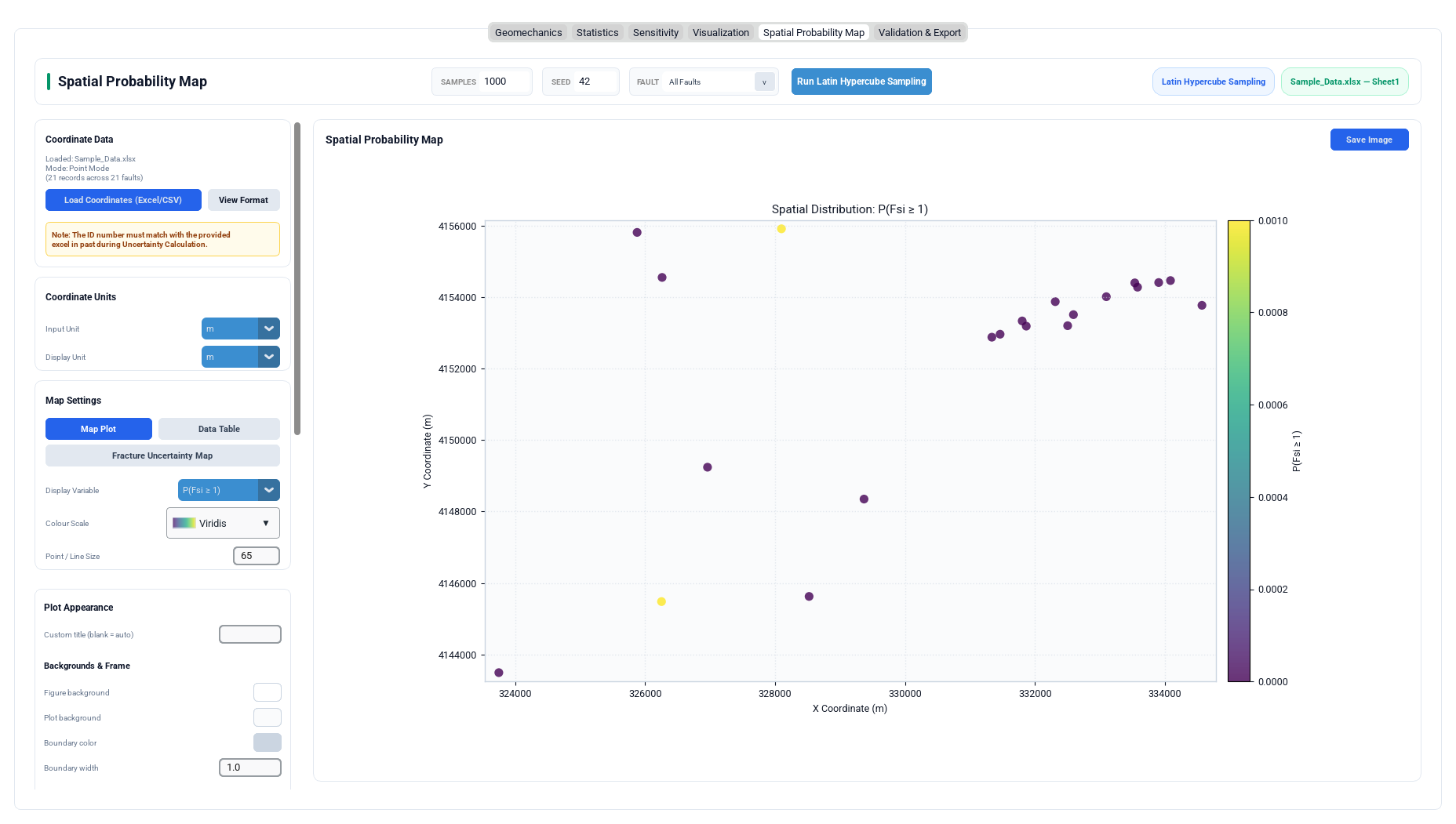
| Load Coordinates | Loads point or trace coordinates from Excel/CSV. |
| View Format | Shows the accepted coordinate layouts and example rows. |
| Input / Display Unit | Controls source and rendered coordinate units independently. |
| Map Plot / Data Table / Fracture Uncertainty Map | Switches the right-hand panel between map, table and uncertainty ranking. |
| Display Variable | P(Fsi ≥ 1), Fsi, P10, P50 or P90. |
| Colour Scale / Point-Line Size | Controls palette and marker/line thickness. |
| Show fault IDs | Annotates points or traces with their identifiers. |
| Export Data | Exports the merged coordinate and statistics table to .xlsx or .csv. |
4.6 Visualization module
Visualization provides response-metric and input selectors, fifteen single-plot types, multiple visualization layouts and a four-panel dashboard. The module also provides KDE and P10–mean–P90 overlays, full-screen viewing, image saving and extensive appearance controls.
5. Mathematical Background
5.1 Latin Hypercube Sampling design
For dimensionality d = 9 and sample size N, LHS partitions the [0,1] probability
range of each dimension into N equal-probability strata. Exactly one sample is taken from every
stratum in each dimension, while the stratum indices are independently permuted between dimensions
(McKay et al., 1979).
FracSTAT generates the design using scipy.stats.qmc.LatinHypercube(d, seed)
(Virtanen et al., 2020).
This produces evenly stratified one-dimensional projections and can reduce sampling variance relative to pseudo-random Monte Carlo at the same sample size, particularly for means of responses dominated by additive input effects (McKay et al., 1979). The benefit depends on the response and statistic: improved precision for every quantile or tail probability is not guaranteed. See Helton and Davis (2003) for uncertainty-propagation applications. The design is a plain Latin hypercube: the strata are permuted independently and no space-filling criterion is optimised over candidate permutations (cf. Morris and Mitchell, 1995), and no rank-correlation structure is induced across dimensions (cf. Iman and Conover, 1982).
5.2 Probability distributions
| Distribution | Parameterisation | Typical use |
|---|---|---|
| Truncated Normal | Requested moments (mean, SD) plus physical bounds [a,b]; the parent normal's μ, σ are solved for | Bounded stress/strength inputs. |
| Normal / Gaussian | μ, σ (unbounded); the same moment-matched Truncated Normal when a finite physical bound applies | Symmetric measurement uncertainty; automatically replaced by Truncated Normal when a finite physical bound applies. |
| Lognormal | Moment-matched μ, σ | Strictly positive, right-skewed quantities. |
| Gamma | Mean and SD converted to shape/scale | Positive quantities with skew controlled by the coefficient of variation. |
| Beta | μ, σ and [lo, hi] | Bounded quantities such as friction coefficient [0,1]. |
| Uniform | [min,max], or bounds derived from μ and σ | Complete lack of preference within a known range. |
Physical bounds are enforced: friction is restricted to [0,1], cohesion and pore pressure are non-negative, and principal stresses are constructed so that all realizations remain non-negative. When a bounded quantity is assigned Normal/Gaussian, the sampler silently uses the equivalent Truncated Normal law and records the effective distribution in reproducibility metadata.
The values entered are the moments of the law that is actually sampled. SciPy's
truncnorm takes loc/scale as the parent normal's μ and σ,
and the truncated distribution's own mean and standard deviation differ from those whenever a bound is
within reach (Johnson, Kotz and Balakrishnan, 1994, Vol. 1, sec. 13.10):
α = (a − μ)/σ,   β = (b − μ)/σ,   Z = Φ(β) − Φ(α)

E[X]   = μ + σ · (φ(α) − φ(β)) / Z

Var[X] = σ² · [ 1 + (α·φ(α) − β·φ(β))/Z − ((φ(α) − φ(β))/Z)² ]
distributions._truncated_normal_parent therefore solves these two relations for the parent
(μ, σ) whose truncation reproduces the requested mean and SD, as nested bracketed root finds: E[X] is
monotone in μ, and the realised SD is then monotone in σ. Both roots are verified before use.
A truncated-normal law cannot carry every (mean, SD) pair: on [0, ∞), SD/mean has a supremum of 1 (the exponential limit); on a finite [a,b], SD cannot exceed (b − a)/√12, with a tighter limit when the mean is away from the midpoint. These are family-specific limits, not limits on every distribution with those bounds. An unattainable request raises an error reporting an approximate attainable SD for the truncated normal rather than quietly sampling different moments. For positive unbounded inputs, consider Lognormal or Gamma; for friction on [0,1], consider Beta or a feasible Uniform law. The alternative must still satisfy its own moment and support constraints.
5.3 Orientation sampling
Strike and SHmax are circular/azimuthal quantities, so a linear normal distribution is unsuitable near the 0°/360° wrap-around. FracSTAT uses the Von Mises distribution (Mardia and Jupp, 2000, ch. 3), where concentration k controls clustering: k = 0 is uniform and larger k produces tighter concentration around the mean.
Dip is bounded to 0–90° and is sampled from a bounded Truncated Normal distribution whose standard deviation is derived from the concentration parameter. Alternatively, Fisher 3D couples Strike and Dip through a single spherical orientation distribution using Strike's concentration parameter (Fisher, 1953).
SHmax always uses its own independent Von Mises concentration because the maximum horizontal stress direction is an independent geomechanical measurement rather than a structural attribute.
5.4 Principal-stress ordering and regime remapping
The sampler guarantees σ1 > σ2 > σ3 by drawing σ3 directly and constructing σ2 and σ1 from σ3 plus two non-negative stress gaps. The configured stress distributions are retained while the gap construction prevents principal-stress crossing. The three regimes follow the Andersonian classification, in which one principal stress is vertical because the free surface carries no shear traction (Anderson, 1951); see also Zoback (2007, ch. 1) for the modern stress-state formulation.
| Regime | Vertical stress | Calculation remap |
|---|---|---|
| Normal Faulting | σ1 | True σ1 is placed in the vertical slot. |
| Strike-Slip | σ2 | True σ2 is placed in the vertical slot. |
| Reverse/Thrust | σ3 | No remap; sampled ordering already matches the calculator convention. |
calculate_fault_stability hard-codes
one geometric assignment — its first argument onto the horizontal axis parallel to SHmax, its second onto
the other horizontal axis, its third onto the vertical — and does not infer a regime. Inside the
calculator the argument names therefore denote slots, not the global maximum and minimum;
only the reverse/thrust case preserves both identities. The displayed and exported ensemble always keeps
the sampled σ1 > σ2 > σ3 columns, and an unrecognised regime string falls back to reverse/thrust.
Because only squared direction cosines enter σn and τ, the permutation changes those scalars by
exactly the intended amount and by nothing else; the regime attribute is recorded on
results.attrs["stress_regime"] for reproducibility.
5.5 Fault-stability equations
For every realization, the downward-directed unit normal (pole) of the fault plane is constructed from strike and dip in an (East, North, Up) frame under the right-hand rule — dip direction = strike + 90°, so the pole trends strike − 90° and plunges 90° − dip — and then projected onto the horizontal principal axes defined by the SHmax azimuth:
n         = ( −sin(dip)·cos(strike),  sin(dip)·sin(strike),  −cos(dip) )

rotated_x = nx·sin(SHmax) + ny·cos(SHmax)        (component along SHmax)
rotated_y = nx·cos(SHmax) − ny·sin(SHmax)        (component along the other horizontal axis)

σn        = σ1·rotated_x² + σ2·rotated_y² + σ3·nz²
|T|²      = σ1²·rotated_x² + σ2²·rotated_y² + σ3²·nz²
τ = √ max(|T|² − σn², 0)| Metric | Formula | Interpretation |
|---|---|---|
| Slip Tendency (Ts) | Ts = τ / σused | Ratio of resolved shear to normal stress; a plane is expected to slip as Ts approaches μ (Morris et al., 1996). |
| Dilation Tendency (Td) | Td = (σ1used − σused) / (σ1used − σ3used) | Normalized tendency for extensional dilation/opening (Ferrill and Morris, 2003). Evaluated from the unpermuted sampled σ1 and σ3 (both reduced by Pp when the effective-stress switch is on), so it is a property of the stress state rather than of the calculator's slot assignment. |
| Fracture Susceptibility (Sf) | Sf = σ′n − (τ − C0) / μ = (σn − Pp) − (τ − C0) / μ | The sustainable pore-pressure increase before the fault reaches the Coulomb criterion, in MPa (Mildren et al., 2002; Streit and Hillis, 2004). Always on effective normal stress — see below. |
| Coulomb Failure Index (Fsi) | Fsi = τ / (C0 + μσused) | Fsi ≥ 1 indicates predicted shear failure on the linear Mohr–Coulomb envelope (Jaeger et al., 2007, ch. 4). |
Effective normal stress is σ′n = σn − Pp, the Terzaghi effective-stress form (Terzaghi, 1943) as applied to faulting by Hubbert and Rubey (1959). The Effective-Stress switch determines whether total or effective stress is used for Ts, Td and Fsi.
The failure flag is Sf ≤ 0, equivalent to the Fsi ≥ 1 criterion, but it is stored as a three-valued boolean: True, False, or missing where Sf could not be evaluated:
result["failure"] = pd.array(
    np.where(np.isfinite(sf_values), sf_values <= 0, None), dtype="boolean"
)np.nan <= 0 is
False, so a plain comparison silently reclassifies every non-evaluable realization — tensile
effective normal stress, zero or negative friction — as "did not fail". Probability of failure, computed as
a mean over the flag, is then biased downwards: the unsafe direction. With the nullable dtype
those rows are excluded from the denominator instead of counted as successes.
5.6 Sensitivity coefficients: SRC and PRCC
SRC is obtained from ordinary least-squares regression of standardized target output against standardized inputs. PRCC measures rank correlation after the effect of all other inputs has been removed in rank space (Iman and Helton, 1988; Marino et al., 2008). Both range from −1 to +1; magnitude indicates relative influence and sign indicates direction.
Two preparation steps are applied to the design matrix before either coefficient is computed.
Strike is folded modulo 180°, because it is axial and the artificial discontinuity at
180°/360° would otherwise enter the regression as if it were real variation in orientation.
Multi-fault population runs are collapsed to one row per realization by
aggregate_paired_faults, so the ranking represents the population rather than one fault's
individual response.
Squared SRCs partition the output variance — that is, they satisfy ΣSRC² = R² and may be read as variance shares — only when the inputs are mutually uncorrelated and the response is linear in them (Iman and Helton, 1988; Saltelli et al., 2008, ch. 1; Marino et al., 2008, sec. 2). Neither condition is guaranteed here: the ordered-gap construction of Section 5.4 can draw σ1, σ2 and σ3 with strong mutual correlation. The module therefore reports three diagnostics with every run — model R², ΣSRC², and the largest |r| between inputs — and adds a warning when |r| > 0.1 and |ΣSRC² − R²| > 0.05 (read the SRCs as conditional regression weights and rank with PRCC instead), or when R² < 0.6 (the response is not well described by a linear model).
5.7 Descriptive and confidence-interval statistics
The Statistics module reports mean, sample standard deviation, median, mode, P10, P50 and P90. The 95% confidence interval of the mean is approximated as:
CI95% = x̄ ± 1.96 × (s / √n)Strike (period 180°, axial) and the SHmax azimuth (period 360°, directional) wrap, so neither has a meaningful arithmetic mean or standard deviation. When one of them is the displayed variable, the location and spread are computed on the circle instead — the mean resultant vector of the angles mapped onto the full circle, with mean = atan2(S, C) and s.d. = √(−2·ln R), scaled back by period/360° (Mardia and Jupp, 2000, sec. 2.2.1, 2.3.2 and 2.3.4; Fisher, 1993, sec. 2.3.1). The P10/mean/P90 overlay on those two inputs is likewise taken on the angular residual about the circular mean, and a band that straddles the wrap point is drawn as the two arcs it actually occupies. Measured on a von Mises sample centred on a true strike of 0.04°, the linear arithmetic mean read 89.89° — the perpendicular orientation; an SHmax azimuth concentrated on 359.98° read 180.28°. Dip is a plunge confined to 0–90° and does not wrap, so it keeps the linear summary.
6. Algorithms
| Algorithm | Implementation / role |
|---|---|
| LHS design generation | sampling_engine._standard_samples uses SciPy's LatinHypercube design and a probit transform. |
| Column alias resolution | _normalise_name, _COLUMN_ALIASES and prepare_faults identify supported input fields. |
| Ordered principal stresses | _sample_inputs constructs σ3 plus non-negative gaps to guarantee σ1 > σ2 > σ3. |
| Distribution transforms | distributions.sample_scalar maps sampled coordinates into physical values; _truncated_normal_parent solves for the parent (μ, σ) that gives a truncated normal the requested moments. |
| Orientation sampling | _von_mises_degrees and _fisher_orientation generate circular or coupled spherical perturbations. |
| Stress-regime remap | _remap_for_regime permutes only which sampled magnitude is passed into each slot of the stability calculator; the exported ensemble keeps σ1 > σ2 > σ3. |
| Fault stability | uncertainty_calculator.calculate_fault_stability performs vectorized stress resolution and metric calculation, including the three-valued failure flag. |
| Sensitivity design matrix | sensitivity.aggregate_paired_faults collapses multi-fault runs to one row per realization and _clean_xy folds strike modulo 180° before fitting; _regression_diagnostics attaches R², ΣSRC² and the largest input |r|. |
| Convergence | validation.convergence_table and convergence_summary evaluate progressively larger nested subsets, attach a bootstrap SEM per checkpoint, and require both a precision and a two-increment stability condition. |
| Clustered standard errors | validation._cluster_bootstrap_standard_errors resamples whole realizations rather than individual fault rows. |
| Analytical benchmarks | validation.analytical_benchmarks checks principal-axis edge cases, with Sf expected on effective normal stress. |
| Reference comparison | validation.reference_comparison compares the vectorized calculator against an independent per-row implementation built from the full stress tensor. |
7. Internal Workflow
7.1 End-to-end run sequence
- Read and validate SAMPLES and SEED.
- Assemble means, standard deviations, distributions, bounds, orientation concentrations, effective-stress setting and stress regime.
- Snapshot the selected fault or the complete fault table for an All-Faults run.
- Disable run/input controls and display the progress overlay.
- Run
sampling_engine.generate_samplesand validation in a daemon worker thread. - Return progress updates to the Qt main thread through
app.after(0, ...). - On success, cache results, refresh the visible module, mark the workspace dirty, autosave and report effective-distribution substitutions.
- On cancellation, restore the idle interface while preserving previous cached results.
- On other exceptions, restore the interface and show the error message.
7.2 Threading and responsiveness
File loading and simulation are performed on background threads. Qt UI updates
are routed through app.after(0, ...), keeping window dragging, tab switching and
cancellation responsive during long simulations.
7.3 Progress reporting
Progress is reported in coarse stages rather than once per realization. The progress workload includes distribution preparation, sampling and stability calculation for each fault, followed by convergence, analytical benchmark, reference comparison and metadata stages.
7.4 Cancellation
A threading.Event is checked at fault-level checkpoints inside
generate_samples. Cancellation is therefore cooperative and normally becomes
effective within roughly one fault's worth of computation.
7.5 Fault-selection caching and effective-stress toggle
Completed results are cached using the active fault-selection label. An existing All-Faults result can be filtered for an individual fault without redundant simulation. The effective-stress switch recalculates Ts, Td, Sf, Fsi and the failure flag for active and cached results without sampling again.
7.6 Autosave
Loading data, switching modes, changing the active module and completing a simulation trigger
silent autosave through core.project_state.save_state. Uncertainty session state
remains independent from Static and Dynamic project state.
8. Statistical Methods and Validation
8.1 Descriptive statistics
Statistics are recalculated whenever the selected metric, input variable or plot type changes. They always use the currently selected fault's cached or freshly computed results.
8.2 Sensitivity analysis
SRC and PRCC populate the numeric sensitivity table and tornado chart. The tornado can be sorted by ascending or descending absolute magnitude or left in input-declaration order. The sidebar note beneath the table always carries the three diagnostics of Section 5.6 — model R², ΣSRC², and the largest |r| between inputs — together with the number of paired samples the fit used.
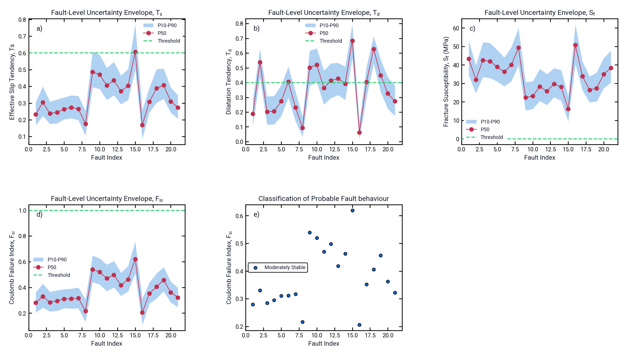
8.3 Fault-level quantile envelopes
per_fault_quantiles groups realizations by fault ID and calculates P10, P50 and P90.
These values define the uncertainty band and central-tendency line used by the Visualization module.
8.4 Validation diagnostics
| Check | Method | Pass criterion |
|---|---|---|
| Nested convergence | Progressively larger nested subsets are evaluated for Ts mean/P50/P90, Sf mean and failure probability. Each checkpoint carries a bootstrap standard error alongside its estimate. | Both conditions, per metric: precision — 1.96 × SEM at the largest level within 2% of the final value (1 percentage point for failure probability); and stability — the last two successive increments both within the same tolerance. Fewer than two levels, or a non-finite SEM, fails. |
| Analytical benchmarks | Principal-axis edge cases are checked against analytically expected values, including Sf on effective normal stress. | Absolute tolerance 1×10⁻¹⁰. |
| Independent tensor reference | Vectorized results are compared with a separate per-row implementation that builds the full stress tensor σ = R·diag(σ1,σ2,σ3)·RT, forms the traction t = σ·n, and takes σn = n·t and τ = ‖t − σn·n‖. | Maximum absolute difference ≤1×10⁻¹⁰. |
Why an increment is not an error bound. The nested levels form a geometric ladder, so a single small step between two neighbouring sizes says only that the estimate happened to move little there. On heavy-tailed synthetic ensembles (Pareto Ts, normal Sf, 40 runs per size) the old final-increment-only rule "passed" 10 of 40 runs at 512 realizations, and 8 of those 10 were still more than 2% away from a 400,000-realization reference; the true remaining error reached 1.9× the increment that had been inspected. The precision condition supplies the missing piece — a Monte Carlo standard error is the actual measure of sampling precision (Helton and Davis, 2003; Saltelli et al., 2008, ch. 2) — while the two-increment stability requirement is the standard successive-refinement check (Roache, 1998, ch. 5).
The standard error resamples realizations, not rows. In a multi-fault run every fault of a
realization shares one sampled stress state, so the rows are clustered and an ordinary row bootstrap would
treat nfaults correlated values as independent evidence and understate the SEM.
_cluster_bootstrap_standard_errors resamples whole realizations with replacement instead
(Efron and Tibshirani, 1993, ch. 8;
Field and Welsh, 2007), using 200 resamples, reduced to 60 above
20,000 rows for runtime; a checkpoint with fewer than two realizations returns NaN. In a single-fault run it
reduces to the ordinary bootstrap.
The reference is deliberately built a different way. The vectorized path uses squared
direction cosines, and that shortcut is exactly what concealed the pole-convention error of
Section 5.5; a reference sharing the same algebra could not have detected it. The tensor
path also computes Sf unconditionally on effective normal stress, matching the calculator. When the
reference instead followed the effective-stress switch, reference_comparison(use_effective_ts=False)
reported a maximum absolute error of 12.0 MPa and "passed": False on a
correctly working calculator. The analytical benchmarks (σ1 = 60, σ2 = 40, σ3 = 25 MPa, Pp = 10, μ = 0.6,
C0 = 0) expect Sf = 15 MPa for a horizontal plane and Sf = 50 MPa for the
vertical case; the previously expected 25 and 60 MPa were the values the buggy calculator produced with Pp
dropped, so the benchmark had been confirming the defect.
9. Visualization
9.1 Geomechanics plots
| Plot | Content |
|---|---|
| Mohr uncertainty diagram | Translucent sampled Mohr circles, mean circles for σ1–σ3, σ1–σ2 and σ2–σ3, and the mean Coulomb envelope. An optional total-stress band provides comparison. |
| Total-stress Mohr circles | Mohr diagram calculated entirely from total stress. |
| Stress scatter | Normal-stress versus shear-stress realizations coloured by Ts, Td or Sf, with optional failure highlighting and Mohr overlays. |
9.2 Statistics plots
| Plot type | Description |
|---|---|
| Metric Histogram | Frequency distribution with mean line and P10–P90 range. |
| Sampled Input Distribution | Distribution of the selected raw input with mean/SD or concentration information. |
| Input-Response Plot | Selected input versus selected metric, colour-mapped by response with a configurable trend curve. |
| Probabilistic Response (Single) | Input histogram with response trend on a second Y axis. |
9.3 Sensitivity tornado
A horizontal bar chart ranks the nine sampled inputs by SRC or PRCC magnitude for the selected target output. A zero-reference line and optional numeric labels can be enabled.
9.4 Spatial Probability Map
Each fault is rendered as a coloured point or line segment and mapped using P(Fsi ≥ 1), mean Fsi, or P10/P50/P90. The companion Fracture Uncertainty Map ranks faults by P90−P10 width, making the least certain outcomes visually prominent.
9.5 Visualization single-plot catalog
| Plot type | Description |
|---|---|
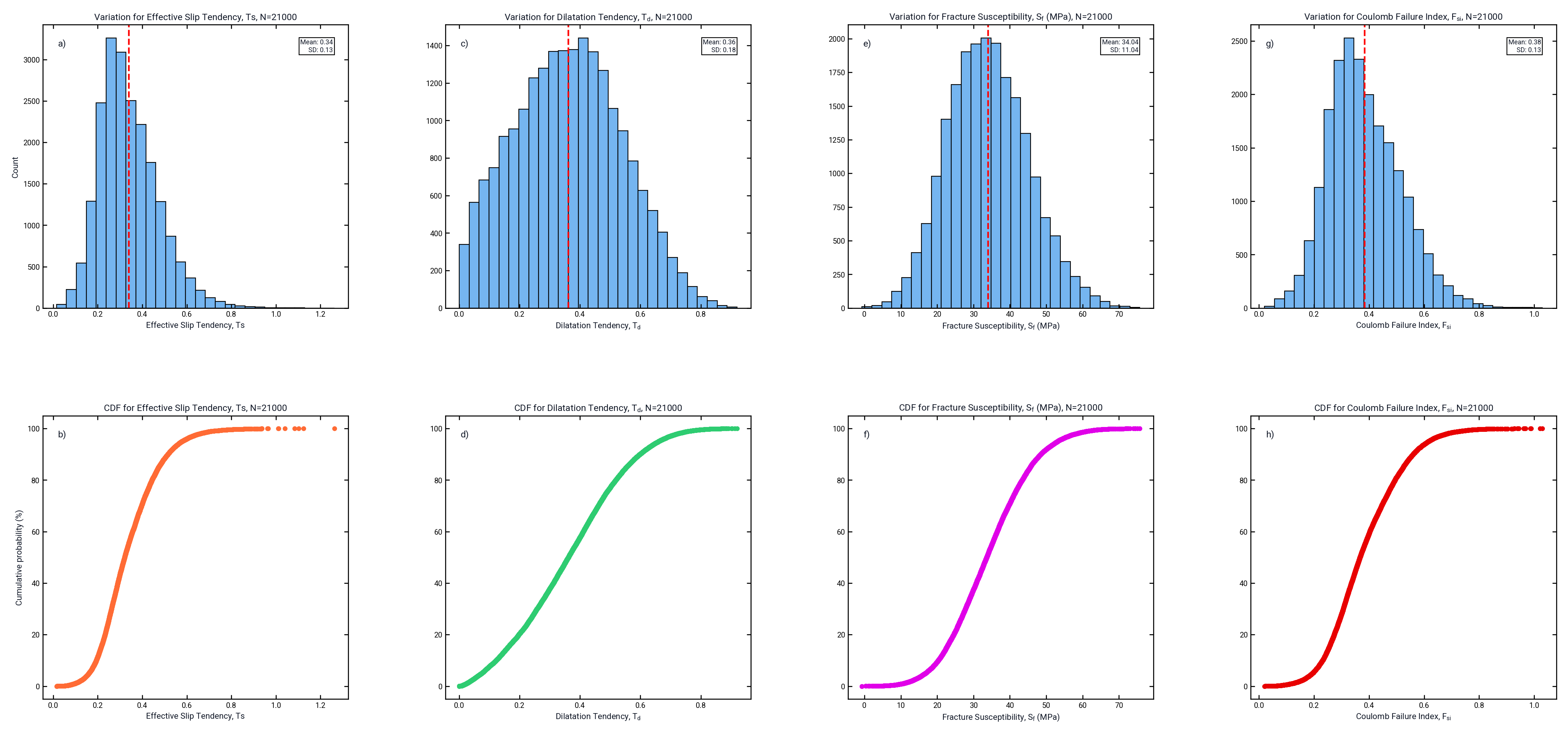
| Histogram / KDE / CDF | Frequency, kernel-density and cumulative-distribution views, with optional fitted Normal PDF. |
| Violin / Box Plot | Distributional comparison of Ts, Td, Sf and Fsi. |
| Ts–Td Density Contours | Bivariate density of Slip Tendency and Dilation Tendency. |
| Ts–Failure Index Relationship | Ts versus Fsi coloured by Td. |
| Input-Response | Input-response relationship with visualization appearance controls. |
| Sampled Input Distribution / Diagnostics | Histogram or density plus empirical-CDF view of an input. |
| Orientation Stereonet | Equal-area lower-hemisphere projection of sampled fault poles. |
| Probabilistic Response | Input distribution and response trend for the selected metric. |
| Sensitivity Tornado | SRC/PRCC ranking with colour-mapped bars. |
| Fault Uncertainty Envelope | Per-fault P10–P90 band and P50 line with metric-specific thresholds. |
| Fault Behaviour Classification | Per-fault P50 Fsi classified as Moderately Stable or Critically Stressed using Fsi ≥ 0.80. |
9.6 Multi-panel layouts
| Layout | Arrangement | Content |
|---|---|---|
| Four-Panel Analysis Dashboard | 2 × 2 | Four independently selectable plot types. |
| Input Parameter Distributions | 2 × 4 | Eight non-fault-ID inputs as annotated histograms. |
| Response Metric Distributions | 2 × 4 | Histogram/CDF pairs for Ts, Td, Sf and Fsi. |
| Probabilistic Response Analysis | 3 × 3 | Eight input-response panels plus a sensitivity tornado. |
| Fault-Level Uncertainty Envelopes | 2 × 3 | Ts, Td, Sf, Fsi envelopes and Fault Behaviour Classification. |
10. Advanced Features
10.1 Full-screen visualization
The Visualization module can detach the active figure into a borderless always-on-top full-screen window with a compact duplicate toolbar. Closing the window restores the same figure inside the embedded canvas.
10.2 Layout editing mode
Move Layout Elements allows plot axes and legends to be click-dragged into custom positions for publication-ready composite figures. Twinned axes belonging to one panel move together.
10.3 Effective vs total stress
This switch changes the physical basis of every Ts, Td and Fsi result across the workspace, while allowing the same sampled realization set to be reused. Sf and the failure flag stay on effective normal stress in either position (Section 5.5), so a comparison run isolates the effect of the basis on the ratio metrics without changing the pore-pressure margin.
10.4 Stress-regime selection
Normal, strike-slip and reverse/thrust Andersonian environments are supported through stress-column remapping without duplicating the underlying stability calculator.
10.5 Fisher 3D orientation sampling
Fisher 3D provides a coupled strike-dip perturbation model when the observed fracture/fault population is better represented by a spherical orientation cluster than two independent one-dimensional distributions.
10.6 Custom plot pixel sizing
Plotting modules expose explicit width and height controls in pixels, allowing figures to be prepared at a specified export resolution or aspect ratio.
11. Performance Optimization
| Technique | Effect |
|---|---|
| Lazy module rendering | Only the visible module is redrawn after a run or fault switch. |
| Fault-result caching | A completed All-Faults run can supply individual fault views without re-simulation. |
| Debounced appearance refresh | Rapid colour/style changes are coalesced into a single redraw. |
| Debounced spatial-map redraw | Map and uncertainty-chart updates are coalesced to avoid repeated colourbar rebuilding. |
| Background-thread simulation and I/O | Keeps the Qt event loop free during CPU- and disk-bound operations. |
| Coarse progress/cancellation checkpoints | Limits thread-boundary overhead while retaining useful cancellation responsiveness. |
| Paginated results table | Only 250 rows are rendered at a time. |
| Selective canvas clearing | Only visible module canvases are cleared/redrawn when necessary. |
| Subsampled Mohr display | Mohr visualization uses a configurable maximum number of representative circles (default 900). |
| Dynamic spatial-map figure sizing | Uncertainty-chart height grows with fault count so labels remain readable. |
12. Practical Examples
12.1 Population-level reactivation screening
- Load the fault orientation workbook with Load Excel/CSV.
- Set the Geomechanics means, SDs and distributions for σ1, σ2, σ3, friction, cohesion, pore pressure and SHmax.
- Leave Strike/Dip means blank when each fault's loaded orientation should be used.
- Select All Faults, choose a sample size such as 5,000, and run LHS.
- Check the Validation & Export convergence card. Increase SAMPLES and repeat if convergence fails.
- Use Visualization → Fault-Level Uncertainty Envelopes to inspect Fsi bands and the Fsi = 1 threshold.
- Load coordinates and use Spatial Probability Map to view P(Fsi ≥ 1) spatially.
12.2 Sensitivity-driven data acquisition
- Select a specific fault and run the LHS sampler.
- Open Sensitivity and choose Ts as the target.
- Use SRC or PRCC to rank the nine inputs.
- Identify the largest-magnitude sensitivity bar as the strongest contributor to Ts variability.
- Prioritize tighter field/laboratory measurement or a reduced uncertainty range for that input in a follow-up run.
12.3 Comparing total and effective stress
- Run with the Effective-Stress switch enabled and record the Fsi distribution.
- Disable the switch. Cached results are recalculated without re-sampling.
- Compare the two Fsi histograms to quantify the effect of pore-pressure assumptions on predicted failure probability.
13. Geological Interpretation
The four response metrics are Mohr–Coulomb fault-mechanics indicators used in reservoir geomechanics, induced-seismicity assessment and structural-diagenesis studies.
13.1 Slip Tendency (Ts)
Ts is the ratio of resolved shear stress to normal stress (Morris et al., 1996). A plane reaches frictional sliding when Ts approaches the static friction coefficient μ. Values around or above approximately 0.6 are commonly treated as near-critical in cohesionless applications, following Byerlee's experimental μ ≈ 0.6–0.85 for most rock types (Byerlee, 1978), but the actual interpretation should follow the friction and cohesion assumptions used in the simulation.
13.2 Dilation Tendency (Td)
Td identifies planes favourably oriented to open under the applied stress state (Ferrill and Morris, 2003). High Td can indicate fracture orientations that are more favourable for dilation and fluid-flow pathways.
13.3 Fracture Susceptibility (Sf)
Sf is expressed in MPa and is read as the pore-pressure increase the fault can sustain before the Coulomb criterion is met at the resolved shear stress (Mildren et al., 2002; Streit and Hillis, 2004): an Sf of 4 MPa means roughly 4 MPa of additional pressure would be expected to reactivate it. Positive Sf indicates a stable margin; Sf ≤ 0 indicates predicted shear failure at current conditions. Because it is a pressure margin it is always computed on effective normal stress, whatever the Effective-Stress switch is set to, and it is reported as missing rather than as a number where it cannot be evaluated (σ′n ≤ 0, or μ ≤ 0).
13.4 Coulomb Failure Index (Fsi)
Fsi is the ratio of resolved shear stress to Mohr–Coulomb frictional strength. Fsi = 1 lies on the failure envelope and Fsi ≥ 1 predicts shear failure. It is the principal metric used by the module's population-level fault-behaviour classification and spatial risk mapping.
13.5 Stress regime and orientation uncertainty
The stress-regime selector follows Andersonian normal, strike-slip and reverse faulting environments. Orientation concentration k provides a way to represent tight or diffuse structural clustering: higher k means a tighter orientation distribution, while lower k represents greater uncertainty. Fisher 3D provides a coupled strike-dip representation where appropriate.
13.6 Why uncertainty quantification matters
Deterministic stability calculations use single best-estimate values and can conceal measurement and interpretive uncertainty. LHS propagates those uncertainties through the same Mohr–Coulomb physics and produces probability distributions, allowing statements such as the probability that a particular fault is critically stressed under the assumed uncertainty model.
14. Implementation Notes
| Topic | Implementation note |
|---|---|
| Shared Monte Carlo code path | uncertainty_lhs_tab.py and uncertainty_montecarlo_tab.py both delegate to UncertaintySamplingTab.build; only the sampling method differs. |
| Standard-normal intermediate representation | Both methods use a common standard-normal coordinate representation before input-specific transforms. |
| Reproducibility metadata | Exports record method, requested/actual sample counts, seed, effective distributions, analysis options, source hash and package versions (Python, NumPy (Harris et al., 2020), pandas (McKinney, 2010), SciPy (Virtanen et al., 2020) and Matplotlib (Hunter, 2007)). |
| Independent session state | Uncertainty state is stored/autosaved separately from Static and Dynamic Analyzer state. |
| Matplotlib integration | Plots are native Matplotlib Figures (Hunter, 2007) embedded using FigureCanvasTkAgg. |
| Matplotlib boxplot compatibility | The Visualization module detects whether the installed Matplotlib version expects labels or tick_labels. |
14.1 Primary Python modules
| Python file | Role |
|---|---|
uncertainty_lhs_tab.py | LHS tab dispatcher; fixes the shared sampling workspace to the LHS method. |
uncertainty_sampling_tab.py | Shared sampling workspace, controls, run orchestration, caching and module views. |
sampling_engine.py | LHS design generation, input sampling, stress ordering, orientation sampling and regime remapping. |
distributions.py | Probability-distribution parameterisation and scalar quantile transforms. |
uncertainty_calculator.py | Vectorized fault-stability calculation and response metrics. |
validation.py | Convergence, analytical benchmark and independent reference diagnostics. |
validation_module.py | Validation & Export user interface and result preview/export handling. |
statistics.py | Descriptive statistics and response statistics. |
sensitivity.py | SRC and PRCC sensitivity calculations. |
spatial_probability_map.py | Coordinate loading, spatial probability rendering and uncertainty ranking. |
visualization.py | Advanced analytical plots, dashboards, appearance controls and image export. |
uncertainty_app.py | Top-level Uncertainty Analyzer application and workspace/session management. |
15. Limitations
- The stability model assumes planar faults with one strike/dip and does not model curvature, roughness or heterogeneous strength along a single fault.
- Cohesion, friction and pore pressure are spatially uniform per fault or population; depth-dependent and spatially varying property models are not implemented.
- Convergence checks combine a bootstrap precision bound with a two-increment stability test on five named metrics (Section 8.4); they are a practical stopping rule for those statistics, not a formal confidence statement about every derived quantity.
- SRC/PRCC can under-represent strongly non-monotonic input-output relationships, and squared SRCs are a variance decomposition only when the inputs are uncorrelated and the response is linear — read the reported R², ΣSRC² and largest input |r| alongside the tornado chart.
- Fracture susceptibility is always computed on effective normal stress and is exempt from the Effective-Stress switch, because a sustainable pore-pressure increase has no total-stress form; it is undefined where σ′n ≤ 0 or μ ≤ 0, and those realizations are excluded from the failure probability rather than counted as non-failures.
- Stress regimes are realised by permuting which sampled magnitude enters each slot of a fixed geometry (Section 5.4), not by re-deriving the geometry; an unrecognised regime string falls back to reverse/thrust.
- A truncated normal cannot reach every (mean, SD) pair: its SD ceiling is (b − a)/√12 on a finite range (lower away from the midpoint), and SD/mean < 1 on [0, ∞). Consider Lognormal or Gamma for positive unbounded inputs, or Beta or a feasible Uniform law for friction on [0,1]; changing the law does not remove its support constraints.
- The ±1.96·s/√n interval on the statistics cards assumes independent, identically distributed rows, which a stratified LHS design pooled across faults does not satisfy; treat it as indicative and use the convergence diagnostics for decisions.
- Circular treatment covers the mean, dispersion and overlay bands of strike and SHmax and the folding of strike before sensitivity fitting; formal circular-uniformity tests (Rayleigh, Watson) on the sampled orientations are not computed.
- Fisher 3D uses one concentration parameter and cannot represent anisotropic elliptical orientation dispersion.
- Spatial mapping requires exact fault-ID matching; fuzzy or partial ID matching is not performed automatically.
- Computation is single-machine and single-process; practical ensemble size is limited by available memory and Matplotlib/Qt rendering responsiveness.
16. References
Sources are listed alphabetically within each group. In-text citations throughout this page link to the corresponding entry below.
16.1 Rock Mechanics, Effective Stress and Fault Stability
- Anderson, E. M. (1951). The Dynamics of Faulting and Dyke Formation with Applications to Britain (2nd ed.). Oliver and Boyd, Edinburgh. (Classification of normal, strike-slip and reverse faulting regimes.)
- Byerlee, J. (1978). Friction of rocks. Pure and Applied Geophysics, 116(4–5), 615–626. https://doi.org/10.1007/BF00876528
- Ferrill, D. A., & Morris, A. P. (2003). Dilational normal faults. Journal of Structural Geology, 25(2), 183–196. https://doi.org/10.1016/S0191-8141(02)00029-9
- Hubbert, M. K., & Rubey, W. W. (1959). Role of fluid pressure in mechanics of overthrust faulting. Geological Society of America Bulletin, 70(2), 115–166. https://doi.org/10.1130/0016-7606(1959)70[115:ROFPIM]2.0.CO;2
- Jaeger, J. C., Cook, N. G. W., & Zimmerman, R. W. (2007). Fundamentals of Rock Mechanics (4th ed.). Blackwell Publishing, Oxford. ISBN 978-0-632-05759-7. (Mohr–Coulomb failure theory, effective stress.)
- Mildren, S. D., Hillis, R. R., & Kaldi, J. (2002). Calibrating predictions of fault seal reactivation in the Timor Sea. The APPEA Journal, 42(1), 187–202. https://doi.org/10.1071/AJ01011
- Morris, A., Ferrill, D. A., & Henderson, D. B. (1996). Slip-tendency analysis and fault reactivation. Geology, 24(3), 275–278. https://doi.org/10.1130/0091-7613(1996)024<0275:STAAFR>2.3.CO;2
- Streit, J. E., & Hillis, R. R. (2004). Estimating fault stability and sustainable fluid pressures for underground storage of CO2 in porous rock. Energy, 29(9–10), 1445–1456. https://doi.org/10.1016/j.energy.2004.03.078
- Terzaghi, K. (1943). Theoretical Soil Mechanics. John Wiley & Sons, New York. https://doi.org/10.1002/9780470172766 (Effective-stress principle.)
- Zoback, M. D. (2007). Reservoir Geomechanics. Cambridge University Press. https://doi.org/10.1017/CBO9780511586477
16.2 Probability Distributions and Directional Statistics
- Fisher, R. A. (1953). Dispersion on a sphere. Proceedings of the Royal Society of London A, 217(1130), 295–305. https://doi.org/10.1098/rspa.1953.0064
- Fisher, N. I. (1993). Statistical Analysis of Circular Data. Cambridge University Press. https://doi.org/10.1017/CBO9780511564345 (Sec. 2.3.1: circular mean and circular standard deviation.)
- Johnson, N. L., Kotz, S., & Balakrishnan, N. (1994). Continuous Univariate Distributions (Vol. 1, 2nd ed.). John Wiley & Sons. ISBN 978-0-471-58495-7. (Sec. 13.10: moments of the truncated normal.)
- Mardia, K. V., & Jupp, P. E. (2000). Directional Statistics. John Wiley & Sons. https://doi.org/10.1002/9780470316979 (Sec. 2.2.1, 2.3.2, 2.3.4 and ch. 3: circular and axial summaries, von Mises law.)
16.3 Sampling, Sensitivity and Convergence
- Efron, B., & Tibshirani, R. J. (1993). An Introduction to the Bootstrap. Chapman & Hall. https://doi.org/10.1007/978-1-4899-4541-9 (Ch. 8: bootstrapping clustered and non-iid data.)
- Field, C. A., & Welsh, A. H. (2007). Bootstrapping clustered data. Journal of the Royal Statistical Society: Series B, 69(3), 369–390. https://doi.org/10.1111/j.1467-9868.2007.00593.x
- Helton, J. C., & Davis, F. J. (2003). Latin hypercube sampling and the propagation of uncertainty in analyses of complex systems. Reliability Engineering & System Safety, 81(1), 23–69. https://doi.org/10.1016/S0951-8320(03)00058-9
- Iman, R. L., & Conover, W. J. (1982). A distribution-free approach to inducing rank correlation among input variables. Communications in Statistics — Simulation and Computation, 11(3), 311–334. https://doi.org/10.1080/03610918208812265
- Iman, R. L., & Helton, J. C. (1988). An investigation of uncertainty and sensitivity analysis techniques for computer models. Risk Analysis, 8(1), 71–90. https://doi.org/10.1111/j.1539-6924.1988.tb01155.x
- Marino, S., Hogue, I. B., Ray, C. J., & Kirschner, D. E. (2008). A methodology for performing global uncertainty and sensitivity analysis in systems biology. Journal of Theoretical Biology, 254(1), 178–196. https://doi.org/10.1016/j.jtbi.2008.04.011
- McKay, M. D., Beckman, R. J., & Conover, W. J. (1979). A comparison of three methods for selecting values of input variables in the analysis of output from a computer code. Technometrics, 21(2), 239–245. https://doi.org/10.2307/1268522
- Morris, M. D., & Mitchell, T. J. (1995). Exploratory designs for computational experiments. Journal of Statistical Planning and Inference, 43(3), 381–402. https://doi.org/10.1016/0378-3758(94)00035-T
- Roache, P. J. (1998). Verification and Validation in Computational Science and Engineering. Hermosa Publishers, Albuquerque. ISBN 978-0-913478-08-0. (Ch. 5: successive-refinement stability as a convergence test.)
- Saltelli, A., Ratto, M., Andres, T., Campolongo, F., Cariboni, J., Gatelli, D., Saisana, M., & Tarantola, S. (2008). Global Sensitivity Analysis: The Primer. John Wiley & Sons. https://doi.org/10.1002/9780470725184
16.4 Software
- Harris, C. R., Millman, K. J., van der Walt, S. J., Gommers, R., Virtanen, P., Cournapeau, D., … Oliphant, T. E. (2020). Array programming with NumPy. Nature, 585(7825), 357–362. https://doi.org/10.1038/s41586-020-2649-2
- Hunter, J. D. (2007). Matplotlib: A 2D graphics environment. Computing in Science & Engineering, 9(3), 90–95. https://doi.org/10.1109/MCSE.2007.55
- McKinney, W. (2010). Data structures for statistical computing in Python. In Proceedings of the 9th Python in Science Conference (pp. 56–61). https://doi.org/10.25080/Majora-92bf1922-00a
- Virtanen, P., Gommers, R., Oliphant, T. E., Haberland, M., Reddy, T., Cournapeau, D., … van Mulbregt, P. (2020). SciPy 1.0: fundamental algorithms for scientific computing in Python. Nature Methods, 17(3), 261–272. https://doi.org/10.1038/s41592-019-0686-2
Methods statement for the LHS tab. If a figure or table produced by this tab appears in a publication, the details below are what a reader needs in order to reproduce it, and are what the citations above assume:
Latin hypercube propagation of stress, strength and orientation uncertainty through the
Mohr–Coulomb fault-stability model
(Jaeger et al., 2007), with N realizations per fault
drawn from a nine-dimensional stratified design
(McKay et al., 1979) generated by
scipy.stats.qmc.LatinHypercube under integer seed s
(SciPy; Virtanen et al., 2020) and mapped to the stated
marginal distributions by inverse CDF; Normal selections on bounded inputs are replaced by
moment-matched truncated normals (Johnson et al., 1994), and
fault orientations are sampled either from independent von Mises laws
(Mardia and Jupp, 2000) or from a coupled Fisher spherical
distribution (Fisher, 1953). Faulting regime follows the
Andersonian classification (Anderson, 1951) and effective
normal stress uses the Terzaghi form
(Terzaghi, 1943;
Hubbert and Rubey, 1959). Reported response metrics are slip
tendency (Morris et al., 1996), dilation tendency
(Ferrill and Morris, 2003), fracture susceptibility
(Mildren et al., 2002;
Streit and Hillis, 2004), and the Coulomb failure index, with
the assumed friction range referenced to laboratory values
(Byerlee, 1978;
Zoback, 2007). Sensitivity is reported as standardized
regression and partial rank correlation coefficients
(Iman and Conover, 1982;
Iman and Helton, 1988;
Saltelli et al., 2008) computed on realization-aggregated
rows, and convergence as a bootstrap precision bound
(Efron and Tibshirani, 1993)
(Helton and Davis, 2003) combined with a successive-refinement
stability test (Roache, 1998). Analyses were run in Python with
NumPy (Harris et al., 2020), pandas
(McKinney, 2010) and Matplotlib
(Hunter, 2007); the exported metadata sheet records the exact
versions, seed and input hash.